优化 (scipy.optimize)

scipy.optimize 包提供了几种常用的优化算法。详细列表可在以下位置找到：scipy.optimize（也可以通过 help(scipy.optimize) 找到）。

多元标量函数的局部极小化 (minimize)

minimize 函数为 scipy.optimize 中多元标量函数的无约束和约束极小化算法提供了一个通用接口。为了演示极小化函数，考虑极小化 \(N\) 变量的 Rosenbrock 函数的问题：

\[f\left(\mathbf{x}\right)=\sum_{i=1}^{N-1}100\left(x_{i+1}-x_{i}^{2}\right)^{2}+\left(1-x_{i}\right)^{2}.\]

当 \(x_{i}=1.\) 时，此函数的最小值为 0。

请注意，Rosenbrock 函数及其导数已包含在 scipy.optimize 中。以下各节所示的实现提供了如何定义目标函数以及其雅可比函数和黑塞函数的示例。scipy.optimize 中的目标函数期望将 numpy 数组作为第一个参数进行优化，并且必须返回一个浮点值。确切的调用签名必须是 f(x, *args)，其中 x 表示一个 numpy 数组，args 是提供给目标函数的附加参数元组。

无约束极小化

Nelder-Mead 单纯形算法 (method='Nelder-Mead')

在下面的示例中，minimize 例程与 Nelder-Mead 单纯形算法（通过 method 参数选择）一起使用。

>>> import numpy as np
>>> from scipy.optimize import minimize

>>> def rosen(x):
...     """The Rosenbrock function"""
...     return sum(100.0*(x[1:]-x[:-1]**2.0)**2.0 + (1-x[:-1])**2.0)

>>> x0 = np.array([1.3, 0.7, 0.8, 1.9, 1.2])
>>> res = minimize(rosen, x0, method='nelder-mead',
...                options={'xatol': 1e-8, 'disp': True})
Optimization terminated successfully.
         Current function value: 0.000000
         Iterations: 339
         Function evaluations: 571

>>> print(res.x)
[1. 1. 1. 1. 1.]

单纯形算法可能是极小化一个行为良好的函数的最简单方法。它只需要函数评估，是简单极小化问题的一个很好的选择。然而，由于它不使用任何梯度评估，因此可能需要更长时间才能找到最小值。

另一种只需要函数调用即可找到最小值的优化算法是 Powell 方法，通过在 minimize 中设置 method='powell' 即可使用。

为了演示如何向目标函数提供附加参数，我们通过附加比例因子 a 和偏移量 b 来极小化 Rosenbrock 函数

\[f\left(\mathbf{x}, a, b\right)=\sum_{i=1}^{N-1}a\left(x_{i+1}-x_{i}^{2}\right)^{2}+\left(1-x_{i}\right)^{2} + b.\]

同样使用 minimize 例程，可以通过以下代码块针对示例参数 a=0.5 和 b=1 解决此问题。

>>> def rosen_with_args(x, a, b):
...     """The Rosenbrock function with additional arguments"""
...     return sum(a*(x[1:]-x[:-1]**2.0)**2.0 + (1-x[:-1])**2.0) + b

>>> x0 = np.array([1.3, 0.7, 0.8, 1.9, 1.2])
>>> res = minimize(rosen_with_args, x0, method='nelder-mead',
...                args=(0.5, 1.), options={'xatol': 1e-8, 'disp': True})
Optimization terminated successfully.
         Current function value: 1.000000
         Iterations: 319 # may vary
         Function evaluations: 525 # may vary

>>> print(res.x)
[1.         1.         1.         1.         0.99999999]

作为使用 minimize 的 args 参数的替代方案，只需将目标函数封装在一个只接受 x 的新函数中。当需要将附加参数作为关键字参数传递给目标函数时，这种方法也很有用。

>>> def rosen_with_args(x, a, *, b):  # b is a keyword-only argument
...     return sum(a*(x[1:]-x[:-1]**2.0)**2.0 + (1-x[:-1])**2.0) + b
>>> def wrapped_rosen_without_args(x):
...     return rosen_with_args(x, 0.5, b=1.)  # pass in `a` and `b`
>>> x0 = np.array([1.3, 0.7, 0.8, 1.9, 1.2])
>>> res = minimize(wrapped_rosen_without_args, x0, method='nelder-mead',
...                options={'xatol': 1e-8,})
>>> print(res.x)
[1.         1.         1.         1.         0.99999999]

另一种替代方案是使用 functools.partial。

>>> from functools import partial
>>> partial_rosen = partial(rosen_with_args, a=0.5, b=1.)
>>> res = minimize(partial_rosen, x0, method='nelder-mead',
...                options={'xatol': 1e-8,})
>>> print(res.x)
[1.         1.         1.         1.         0.99999999]

Broyden-Fletcher-Goldfarb-Shanno 算法 (method='BFGS')

为了更快地收敛到解决方案，此例程使用目标函数的梯度。如果用户未提供梯度，则使用一阶差分进行估计。Broyden-Fletcher-Goldfarb-Shanno (BFGS) 方法通常比单纯形算法需要更少的函数调用，即使在必须估计梯度的情况下也是如此。

为了演示此算法，再次使用 Rosenbrock 函数。Rosenbrock 函数的梯度是向量

\begin{eqnarray*} \frac{\partial f}{\partial x_{j}} & = & \sum_{i=1}^{N}200\left(x_{i}-x_{i-1}^{2}\right)\left(\delta_{i,j}-2x_{i-1}\delta_{i-1,j}\right)-2\left(1-x_{i-1}\right)\delta_{i-1,j}.\\ & = & 200\left(x_{j}-x_{j-1}^{2}\right)-400x_{j}\left(x_{j+1}-x_{j}^{2}\right)-2\left(1-x_{j}\right).\end{eqnarray*}

此表达式对内部导数有效。特殊情况是

\begin{eqnarray*} \frac{\partial f}{\partial x_{0}} & = & -400x_{0}\left(x_{1}-x_{0}^{2}\right)-2\left(1-x_{0}\right),\\ \frac{\partial f}{\partial x_{N-1}} & = & 200\left(x_{N-1}-x_{N-2}^{2}\right).\end{eqnarray*}

计算此梯度的 Python 函数由代码片段构建

>>> def rosen_der(x):
...     xm = x[1:-1]
...     xm_m1 = x[:-2]
...     xm_p1 = x[2:]
...     der = np.zeros_like(x)
...     der[1:-1] = 200*(xm-xm_m1**2) - 400*(xm_p1 - xm**2)*xm - 2*(1-xm)
...     der[0] = -400*x[0]*(x[1]-x[0]**2) - 2*(1-x[0])
...     der[-1] = 200*(x[-1]-x[-2]**2)
...     return der

此梯度信息在 minimize 函数中通过 jac 参数指定，如下所示。

>>> res = minimize(rosen, x0, method='BFGS', jac=rosen_der,
...                options={'disp': True})
Optimization terminated successfully.
         Current function value: 0.000000
         Iterations: 25                     # may vary
         Function evaluations: 30
         Gradient evaluations: 30
>>> res.x
array([1., 1., 1., 1., 1.])

避免冗余计算

目标函数及其梯度通常共享计算的某些部分。例如，考虑以下问题。

>>> def f(x):
...    return -expensive(x[0])**2
>>>
>>> def df(x):
...     return -2 * expensive(x[0]) * dexpensive(x[0])
>>>
>>> def expensive(x):
...     # this function is computationally expensive!
...     expensive.count += 1  # let's keep track of how many times it runs
...     return np.sin(x)
>>> expensive.count = 0
>>>
>>> def dexpensive(x):
...     return np.cos(x)
>>>
>>> res = minimize(f, 0.5, jac=df)
>>> res.fun
-0.9999999999999174
>>> res.nfev, res.njev
6, 6
>>> expensive.count
12

这里，expensive 被调用了 12 次：在目标函数中调用了 6 次，从梯度中调用了 6 次。减少冗余计算的一种方法是创建一个返回目标函数和梯度的单个函数。

>>> def f_and_df(x):
...     expensive_value = expensive(x[0])
...     return (-expensive_value**2,  # objective function
...             -2*expensive_value*dexpensive(x[0]))  # gradient
>>>
>>> expensive.count = 0  # reset the counter
>>> res = minimize(f_and_df, 0.5, jac=True)
>>> res.fun
-0.9999999999999174
>>> expensive.count
6

当我们调用 minimize 时，我们指定 jac==True 以指示提供的函数同时返回目标函数及其梯度。虽然方便，但并非所有 scipy.optimize 函数都支持此功能，而且它仅用于在函数及其梯度之间共享计算，而在某些问题中，我们希望与 Hessian（目标函数的二阶导数）和约束共享计算。更通用的方法是记忆计算中的昂贵部分。在简单情况下，这可以通过 functools.lru_cache 包装器实现。

>>> from functools import lru_cache
>>> expensive.count = 0  # reset the counter
>>> expensive = lru_cache(expensive)
>>> res = minimize(f, 0.5, jac=df)
>>> res.fun
-0.9999999999999174
>>> expensive.count
6

牛顿共轭梯度算法 (method='Newton-CG')

牛顿共轭梯度算法是牛顿法的改进版本，它使用共轭梯度算法来（近似）反转局部黑塞矩阵 [NW]。牛顿法基于将函数局部拟合为二次形式：

\[f\left(\mathbf{x}\right)\approx f\left(\mathbf{x}_{0}\right)+\nabla f\left(\mathbf{x}_{0}\right)\cdot\left(\mathbf{x}-\mathbf{x}_{0}\right)+\frac{1}{2}\left(\mathbf{x}-\mathbf{x}_{0}\right)^{T}\mathbf{H}\left(\mathbf{x}_{0}\right)\left(\mathbf{x}-\mathbf{x}_{0}\right).\]

其中 \(\mathbf{H}\left(\mathbf{x}_{0}\right)\) 是二阶导数矩阵（黑塞矩阵）。如果黑塞矩阵是正定的，则可以通过将二次形式的梯度设为零来找到此函数的局部最小值，从而得到

\[\mathbf{x}_{\textrm{opt}}=\mathbf{x}_{0}-\mathbf{H}^{-1}\nabla f.\]

黑塞矩阵的逆使用共轭梯度法进行评估。下面给出了将此方法应用于极小化 Rosenbrock 函数的示例。为了充分利用牛顿-CG 方法，必须提供计算黑塞矩阵的函数。黑塞矩阵本身不需要构建，只需要计算黑塞矩阵与任意向量乘积的函数即可用于极小化例程。因此，用户可以提供计算黑塞矩阵的函数，也可以提供计算黑塞矩阵与任意向量乘积的函数。

完整黑塞矩阵示例

Rosenbrock 函数的黑塞矩阵是

\begin{eqnarray*} H_{ij}=\frac{\partial^{2}f}{\partial x_{i}\partial x_{j}} & = & 200\left(\delta_{i,j}-2x_{i-1}\delta_{i-1,j}\right)-400x_{i}\left(\delta_{i+1,j}-2x_{i}\delta_{i,j}\right)-400\delta_{i,j}\left(x_{i+1}-x_{i}^{2}\right)+2\delta_{i,j},\\ & = & \left(202+1200x_{i}^{2}-400x_{i+1}\right)\delta_{i,j}-400x_{i}\delta_{i+1,j}-400x_{i-1}\delta_{i-1,j},\end{eqnarray*}

如果 \(i,j\in\left[1,N-2\right]\) 且 \(i,j\in\left[0,N-1\right]\) 定义了 \(N\times N\) 矩阵。矩阵的其他非零项是

\begin{eqnarray*} \frac{\partial^{2}f}{\partial x_{0}^{2}} & = & 1200x_{0}^{2}-400x_{1}+2,\\ \frac{\partial^{2}f}{\partial x_{0}\partial x_{1}}=\frac{\partial^{2}f}{\partial x_{1}\partial x_{0}} & = & -400x_{0},\\ \frac{\partial^{2}f}{\partial x_{N-1}\partial x_{N-2}}=\frac{\partial^{2}f}{\partial x_{N-2}\partial x_{N-1}} & = & -400x_{N-2},\\ \frac{\partial^{2}f}{\partial x_{N-1}^{2}} & = & 200.\end{eqnarray*}

例如，当 \(N=5\) 时的黑塞矩阵是

\[\begin{split}\mathbf{H}=\begin{bmatrix} 1200x_{0}^{2}+2\mkern-2em\\&1200x_{1}^{2}+202\mkern-2em\\&&1200x_{1}^{2}+202\mkern-2em\\&&&1200x_{3}^{2}+202\mkern-1em\\&&&&200\end{bmatrix}-400\begin{bmatrix} x_1 & x_0 \\ x_0 & x_2 & x_1 \\ & x_1 & x_3 & x_2\\ & & x_2 & x_4 & x_3 \\ & & & x_3 & 0\end{bmatrix}.\end{split}\]

计算此黑塞矩阵以及使用牛顿-CG 方法极小化函数的代码在以下示例中显示

>>> def rosen_hess(x):
...     x = np.asarray(x)
...     H = np.diag(-400*x[:-1],1) - np.diag(400*x[:-1],-1)
...     diagonal = np.zeros_like(x)
...     diagonal[0] = 1200*x[0]**2-400*x[1]+2
...     diagonal[-1] = 200
...     diagonal[1:-1] = 202 + 1200*x[1:-1]**2 - 400*x[2:]
...     H = H + np.diag(diagonal)
...     return H

>>> res = minimize(rosen, x0, method='Newton-CG',
...                jac=rosen_der, hess=rosen_hess,
...                options={'xtol': 1e-8, 'disp': True})
Optimization terminated successfully.
         Current function value: 0.000000
         Iterations: 19                       # may vary
         Function evaluations: 22
         Gradient evaluations: 19
         Hessian evaluations: 19
>>> res.x
array([1.,  1.,  1.,  1.,  1.])

黑塞积示例

对于较大的极小化问题，存储整个黑塞矩阵会消耗大量时间和内存。牛顿-CG 算法只需要黑塞矩阵乘以任意向量的积。因此，用户可以提供计算此积的代码，而不是完整的黑塞矩阵，方法是提供一个 hess 函数，该函数将极小化向量作为第一个参数，将任意向量作为第二个参数（以及传递给要极小化函数的额外参数）。如果可能，使用带有黑塞积选项的牛顿-CG 可能是极小化函数的最快方法。

在这种情况下，Rosenbrock 黑塞矩阵与任意向量的积并不难计算。如果 \(\mathbf{p}\) 是任意向量，则 \(\mathbf{H}\left(\mathbf{x}\right)\mathbf{p}\) 的元素是

\[\begin{split}\mathbf{H}\left(\mathbf{x}\right)\mathbf{p}=\begin{bmatrix} \left(1200x_{0}^{2}-400x_{1}+2\right)p_{0}-400x_{0}p_{1}\\ \vdots\\ -400x_{i-1}p_{i-1}+\left(202+1200x_{i}^{2}-400x_{i+1}\right)p_{i}-400x_{i}p_{i+1}\\ \vdots\\ -400x_{N-2}p_{N-2}+200p_{N-1}\end{bmatrix}.\end{split}\]

下面是使用此黑塞积通过 minimize 极小化 Rosenbrock 函数的代码

>>> def rosen_hess_p(x, p):
...     x = np.asarray(x)
...     Hp = np.zeros_like(x)
...     Hp[0] = (1200*x[0]**2 - 400*x[1] + 2)*p[0] - 400*x[0]*p[1]
...     Hp[1:-1] = -400*x[:-2]*p[:-2]+(202+1200*x[1:-1]**2-400*x[2:])*p[1:-1] \
...                -400*x[1:-1]*p[2:]
...     Hp[-1] = -400*x[-2]*p[-2] + 200*p[-1]
...     return Hp

>>> res = minimize(rosen, x0, method='Newton-CG',
...                jac=rosen_der, hessp=rosen_hess_p,
...                options={'xtol': 1e-8, 'disp': True})
Optimization terminated successfully.
         Current function value: 0.000000
         Iterations: 20                    # may vary
         Function evaluations: 23
         Gradient evaluations: 20
         Hessian evaluations: 44
>>> res.x
array([1., 1., 1., 1., 1.])

根据 [NW] 第 170 页，当黑塞矩阵病态时，Newton-CG 算法可能效率低下，因为该方法在这些情况下提供的搜索方向质量较差。作者表示，trust-ncg 方法能更有效地处理这种有问题的情况，接下来将进行描述。

信赖域牛顿共轭梯度算法 (method='trust-ncg')

Newton-CG 方法是一种线搜索方法：它找到一个搜索方向，使函数的二次近似最小化，然后使用线搜索算法找到该方向上（接近）最优的步长。另一种方法是，首先，固定步长限制 \(\Delta\)，然后通过求解以下二次子问题来找到给定信赖半径内的最优步长 \(\mathbf{p}\)：

\begin{eqnarray*} \min_{\mathbf{p}} f\left(\mathbf{x}_{k}\right)+\nabla f\left(\mathbf{x}_{k}\right)\cdot\mathbf{p}+\frac{1}{2}\mathbf{p}^{T}\mathbf{H}\left(\mathbf{x}_{k}\right)\mathbf{p};&\\ \text{subject to: } \|\mathbf{p}\|\le \Delta.& \end{eqnarray*}

然后更新解 \(\mathbf{x}_{k+1} = \mathbf{x}_{k} + \mathbf{p}\)，并根据二次模型与实际函数的一致程度调整信赖半径 \(\Delta\)。这类方法被称为信赖域方法。trust-ncg 算法是一种信赖域方法，它使用共轭梯度算法来求解信赖域子问题 [NW]。

完整黑塞矩阵示例

>>> res = minimize(rosen, x0, method='trust-ncg',
...                jac=rosen_der, hess=rosen_hess,
...                options={'gtol': 1e-8, 'disp': True})
Optimization terminated successfully.
         Current function value: 0.000000
         Iterations: 20                    # may vary
         Function evaluations: 21
         Gradient evaluations: 20
         Hessian evaluations: 19
>>> res.x
array([1., 1., 1., 1., 1.])

黑塞积示例

>>> res = minimize(rosen, x0, method='trust-ncg',
...                jac=rosen_der, hessp=rosen_hess_p,
...                options={'gtol': 1e-8, 'disp': True})
Optimization terminated successfully.
         Current function value: 0.000000
         Iterations: 20                    # may vary
         Function evaluations: 21
         Gradient evaluations: 20
         Hessian evaluations: 0
>>> res.x
array([1., 1., 1., 1., 1.])

信赖域截断广义 Lanczos / 共轭梯度算法 (method='trust-krylov')

与 trust-ncg 方法类似，trust-krylov 方法适用于大规模问题，因为它仅通过矩阵-向量乘积将黑塞矩阵用作线性算子。它比 trust-ncg 方法更准确地解决二次子问题。

\begin{eqnarray*} \min_{\mathbf{p}} f\left(\mathbf{x}_{k}\right)+\nabla f\left(\mathbf{x}_{k}\right)\cdot\mathbf{p}+\frac{1}{2}\mathbf{p}^{T}\mathbf{H}\left(\mathbf{x}_{k}\right)\mathbf{p};&\\ \text{subject to: } \|\mathbf{p}\|\le \Delta.& \end{eqnarray*}

此方法封装了 [TRLIB] 实现的 [GLTR] 方法，该方法精确求解了受截断 Krylov 子空间限制的信赖域子问题。对于不定问题，通常最好使用此方法，因为它与 trust-ncg 方法相比，以每个子问题求解的少量矩阵-向量乘积为代价，减少了非线性迭代的次数。

完整黑塞矩阵示例

>>> res = minimize(rosen, x0, method='trust-krylov',
...                jac=rosen_der, hess=rosen_hess,
...                options={'gtol': 1e-8, 'disp': True})
Optimization terminated successfully.
         Current function value: 0.000000
         Iterations: 19                    # may vary
         Function evaluations: 20
         Gradient evaluations: 20
         Hessian evaluations: 18
>>> res.x
array([1., 1., 1., 1., 1.])

黑塞积示例

>>> res = minimize(rosen, x0, method='trust-krylov',
...                jac=rosen_der, hessp=rosen_hess_p,
...                options={'gtol': 1e-8, 'disp': True})
Optimization terminated successfully.
         Current function value: 0.000000
         Iterations: 19                    # may vary
         Function evaluations: 20
         Gradient evaluations: 20
         Hessian evaluations: 0
>>> res.x
array([1., 1., 1., 1., 1.])

[TRLIB]

F. Lenders, C. Kirches, A. Potschka: "trlib: A vector-free implementation of the GLTR method for iterative solution of the trust region problem", arXiv:1611.04718

[GLTR]

N. Gould, S. Lucidi, M. Roma, P. Toint: "Solving the Trust-Region Subproblem using the Lanczos Method", SIAM J. Optim., 9(2), 504–525, (1999). DOI:10.1137/S1052623497322735

信赖域近乎精确算法 (method='trust-exact')

所有方法 Newton-CG、trust-ncg 和 trust-krylov 都适用于处理大规模问题（具有数千个变量的问题）。这是因为共轭梯度算法通过迭代近似求解信赖域子问题（或反转黑塞矩阵），而无需明确的黑塞矩阵因式分解。由于只需要黑塞矩阵与任意向量的乘积，因此该算法特别适合处理稀疏黑塞矩阵，从而为这些稀疏问题节省了存储需求和大量时间。

对于中等规模问题，即黑塞矩阵的存储和分解成本不重要的场景，可以通过几乎精确地求解信赖域子问题，在更少的迭代次数内获得解。为此，对于每个二次子问题，都会迭代求解某个非线性方程 [CGT]。此解通常需要对黑塞矩阵进行 3 到 4 次 Cholesky 分解。因此，该方法比其他已实现的信赖域方法收敛得更快，并且目标函数评估次数更少。此算法不支持黑塞积选项。下面是使用 Rosenbrock 函数的示例

>>> res = minimize(rosen, x0, method='trust-exact',
...                jac=rosen_der, hess=rosen_hess,
...                options={'gtol': 1e-8, 'disp': True})
Optimization terminated successfully.
         Current function value: 0.000000
         Iterations: 13                    # may vary
         Function evaluations: 14
         Gradient evaluations: 13
         Hessian evaluations: 14
>>> res.x
array([1., 1., 1., 1., 1.])

[NW] (1,2,3)

J. Nocedal, S.J. Wright "数值优化" 第二版. Springer Science (2006)。

[CGT]

Conn, A. R., Gould, N. I., & Toint, P. L. "信赖域方法". Siam. (2000). pp. 169-200.

受约束极小化

minimize 函数提供了几种用于约束极小化的算法，即 'trust-constr'、'SLSQP'、'COBYLA' 和 'COBYQA'。它们要求约束使用略微不同的结构定义。方法 'trust-constr'、'COBYQA' 和 'COBYLA' 要求将约束定义为 LinearConstraint 和 NonlinearConstraint 对象的序列。另一方面，方法 'SLSQP' 要求将约束定义为字典序列，键为 type、fun 和 jac。

例如，让我们考虑 Rosenbrock 函数的约束极小化

\begin{eqnarray*} \min_{x_0, x_1} & ~~100\left(x_{1}-x_{0}^{2}\right)^{2}+\left(1-x_{0}\right)^{2} &\\ \text{subject to: } & x_0 + 2 x_1 \leq 1 & \\ & x_0^2 + x_1 \leq 1 & \\ & x_0^2 - x_1 \leq 1 & \\ & 2 x_0 + x_1 = 1 & \\ & 0 \leq x_0 \leq 1 & \\ & -0.5 \leq x_1 \leq 2.0. & \end{eqnarray*}

此优化问题具有唯一解 \([x_0, x_1] = [0.4149,~ 0.1701]\)，其中只有第一个和第四个约束是活跃的。

信赖域约束算法 (method='trust-constr')

信赖域约束方法处理以下形式的约束极小化问题

\begin{eqnarray*} \min_x & f(x) & \\ \text{subject to: } & ~~~ c^l \leq c(x) \leq c^u, &\\ & x^l \leq x \leq x^u. & \end{eqnarray*}

当 \(c^l_j = c^u_j\) 时，该方法将第 \(j\) 个约束视为等式约束并相应地处理。此外，可以通过将上限或下限设置为具有适当符号的 np.inf 来指定单侧约束。

该实现基于等式约束问题的 [EQSQP] 和不等式约束问题的 [TRIP]。两者都是适用于大规模问题的信赖域类型算法。

定义边界约束

边界约束 \(0 \leq x_0 \leq 1\) 和 \(-0.5 \leq x_1 \leq 2.0\) 使用 Bounds 对象定义。

>>> from scipy.optimize import Bounds
>>> bounds = Bounds([0, -0.5], [1.0, 2.0])

定义线性约束

约束 \(x_0 + 2 x_1 \leq 1\) 和 \(2 x_0 + x_1 = 1\) 可以写成线性约束标准格式

\begin{equation*} \begin{bmatrix}-\infty \\1\end{bmatrix} \leq \begin{bmatrix} 1& 2 \\ 2& 1\end{bmatrix} \begin{bmatrix} x_0 \\x_1\end{bmatrix} \leq \begin{bmatrix} 1 \\ 1\end{bmatrix},\end{equation*}

并使用 LinearConstraint 对象定义。

>>> from scipy.optimize import LinearConstraint
>>> linear_constraint = LinearConstraint([[1, 2], [2, 1]], [-np.inf, 1], [1, 1])

定义非线性约束 非线性约束

\begin{equation*} c(x) = \begin{bmatrix} x_0^2 + x_1 \\ x_0^2 - x_1\end{bmatrix} \leq \begin{bmatrix} 1 \\ 1\end{bmatrix}, \end{equation*}

以及雅可比矩阵

\begin{equation*} J(x) = \begin{bmatrix} 2x_0 & 1 \\ 2x_0 & -1\end{bmatrix},\end{equation*}

和黑塞矩阵的线性组合

\begin{equation*} H(x, v) = \sum_{i=0}^1 v_i \nabla^2 c_i(x) = v_0\begin{bmatrix} 2 & 0 \\ 0 & 0\end{bmatrix} + v_1\begin{bmatrix} 2 & 0 \\ 0 & 0\end{bmatrix}, \end{equation*}

使用 NonlinearConstraint 对象定义。

>>> def cons_f(x):
...     return [x[0]**2 + x[1], x[0]**2 - x[1]]
>>> def cons_J(x):
...     return [[2*x[0], 1], [2*x[0], -1]]
>>> def cons_H(x, v):
...     return v[0]*np.array([[2, 0], [0, 0]]) + v[1]*np.array([[2, 0], [0, 0]])
>>> from scipy.optimize import NonlinearConstraint
>>> nonlinear_constraint = NonlinearConstraint(cons_f, -np.inf, 1, jac=cons_J, hess=cons_H)

或者，也可以将黑塞矩阵 \(H(x, v)\) 定义为稀疏矩阵，

>>> from scipy.sparse import csc_matrix
>>> def cons_H_sparse(x, v):
...     return v[0]*csc_matrix([[2, 0], [0, 0]]) + v[1]*csc_matrix([[2, 0], [0, 0]])
>>> nonlinear_constraint = NonlinearConstraint(cons_f, -np.inf, 1,
...                                            jac=cons_J, hess=cons_H_sparse)

或作为 LinearOperator 对象。

>>> from scipy.sparse.linalg import LinearOperator
>>> def cons_H_linear_operator(x, v):
...     def matvec(p):
...         return np.array([p[0]*2*(v[0]+v[1]), 0])
...     return LinearOperator((2, 2), matvec=matvec)
>>> nonlinear_constraint = NonlinearConstraint(cons_f, -np.inf, 1,
...                                           jac=cons_J, hess=cons_H_linear_operator)

当黑塞矩阵 \(H(x, v)\) 的评估难以实现或计算上不可行时，可以使用 HessianUpdateStrategy。目前可用的策略是 BFGS 和 SR1。

>>> from scipy.optimize import BFGS
>>> nonlinear_constraint = NonlinearConstraint(cons_f, -np.inf, 1, jac=cons_J, hess=BFGS())

或者，黑塞矩阵可以使用有限差分进行近似。

>>> nonlinear_constraint = NonlinearConstraint(cons_f, -np.inf, 1, jac=cons_J, hess='2-point')

约束的雅可比矩阵也可以通过有限差分近似。然而，在这种情况下，黑塞矩阵不能用有限差分计算，需要由用户提供或使用 HessianUpdateStrategy 定义。

>>> nonlinear_constraint = NonlinearConstraint(cons_f, -np.inf, 1, jac='2-point', hess=BFGS())

求解优化问题 优化问题通过以下方式求解

>>> x0 = np.array([0.5, 0])
>>> res = minimize(rosen, x0, method='trust-constr', jac=rosen_der, hess=rosen_hess,
...                constraints=[linear_constraint, nonlinear_constraint],
...                options={'verbose': 1}, bounds=bounds)
# may vary
`gtol` termination condition is satisfied.
Number of iterations: 12, function evaluations: 8, CG iterations: 7, optimality: 2.99e-09, constraint violation: 1.11e-16, execution time: 0.016 s.
>>> print(res.x)
[0.41494531 0.17010937]

当需要时，目标函数的黑塞矩阵可以使用 LinearOperator 对象定义，

>>> def rosen_hess_linop(x):
...     def matvec(p):
...         return rosen_hess_p(x, p)
...     return LinearOperator((2, 2), matvec=matvec)
>>> res = minimize(rosen, x0, method='trust-constr', jac=rosen_der, hess=rosen_hess_linop,
...                constraints=[linear_constraint, nonlinear_constraint],
...                options={'verbose': 1}, bounds=bounds)
# may vary
`gtol` termination condition is satisfied.
Number of iterations: 12, function evaluations: 8, CG iterations: 7, optimality: 2.99e-09, constraint violation: 1.11e-16, execution time: 0.018 s.
>>> print(res.x)
[0.41494531 0.17010937]

或通过参数 hessp 进行 Hessian-向量乘积。

>>> res = minimize(rosen, x0, method='trust-constr', jac=rosen_der, hessp=rosen_hess_p,
...                constraints=[linear_constraint, nonlinear_constraint],
...                options={'verbose': 1}, bounds=bounds)
# may vary
`gtol` termination condition is satisfied.
Number of iterations: 12, function evaluations: 8, CG iterations: 7, optimality: 2.99e-09, constraint violation: 1.11e-16, execution time: 0.018 s.
>>> print(res.x)
[0.41494531 0.17010937]

或者，目标函数的一阶和二阶导数可以近似。例如，Hessian 可以用 SR1 拟牛顿近似，梯度可以用有限差分。

>>> from scipy.optimize import SR1
>>> res = minimize(rosen, x0, method='trust-constr',  jac="2-point", hess=SR1(),
...                constraints=[linear_constraint, nonlinear_constraint],
...                options={'verbose': 1}, bounds=bounds)
# may vary
`gtol` termination condition is satisfied.
Number of iterations: 12, function evaluations: 24, CG iterations: 7, optimality: 4.48e-09, constraint violation: 0.00e+00, execution time: 0.016 s.
>>> print(res.x)
[0.41494531 0.17010937]

[TRIP]

Byrd, Richard H., Mary E. Hribar, and Jorge Nocedal. 1999. 一种用于大规模非线性规划的内点算法。SIAM Journal on Optimization 9.4: 877-900。

[EQSQP]

Lalee, Marucha, Jorge Nocedal, and Todd Plantega. 1998. 大规模等式约束优化算法的实现。SIAM Journal on Optimization 8.3: 682-706。

序列最小二乘规划 (SLSQP) 算法 (method='SLSQP')

SLSQP 方法处理以下形式的约束极小化问题

\begin{eqnarray*} \min_x & f(x) \\ \text{subject to: } & c_j(x) = 0 , &j \in \mathcal{E}\\ & c_j(x) \geq 0 , &j \in \mathcal{I}\\ & \text{lb}_i \leq x_i \leq \text{ub}_i , &i = 1,...,N. \end{eqnarray*}

其中 \(\mathcal{E}\) 或 \(\mathcal{I}\) 是包含等式和不等式约束的索引集。

线性和非线性约束都定义为带有键 type、fun 和 jac 的字典。

>>> ineq_cons = {'type': 'ineq',
...              'fun' : lambda x: np.array([1 - x[0] - 2*x[1],
...                                          1 - x[0]**2 - x[1],
...                                          1 - x[0]**2 + x[1]]),
...              'jac' : lambda x: np.array([[-1.0, -2.0],
...                                          [-2*x[0], -1.0],
...                                          [-2*x[0], 1.0]])}
>>> eq_cons = {'type': 'eq',
...            'fun' : lambda x: np.array([2*x[0] + x[1] - 1]),
...            'jac' : lambda x: np.array([2.0, 1.0])}

并且优化问题通过以下方式求解

>>> x0 = np.array([0.5, 0])
>>> res = minimize(rosen, x0, method='SLSQP', jac=rosen_der,
...                constraints=[eq_cons, ineq_cons], options={'ftol': 1e-9, 'disp': True},
...                bounds=bounds)
# may vary
Optimization terminated successfully.    (Exit mode 0)
            Current function value: 0.342717574857755
            Iterations: 5
            Function evaluations: 6
            Gradient evaluations: 5
>>> print(res.x)
[0.41494475 0.1701105 ]

方法 'trust-constr' 的大部分可用选项不适用于 'SLSQP'。

局部极小化求解器比较

使用下表查找满足您要求的求解器。如果有多个候选者，请尝试几个并查看哪个最能满足您的需求（例如，执行时间、目标函数值）。

求解器	边界约束	非线性约束	使用梯度	使用黑塞矩阵	利用稀疏性
CG			✓
BFGS			✓
dogleg			✓	✓
trust-ncg			✓	✓
trust-krylov			✓	✓
trust-exact			✓	✓
Newton-CG			✓	✓	✓
Nelder-Mead	✓
Powell	✓
L-BFGS-B	✓		✓
TNC	✓		✓
COBYLA	✓	✓
COBYQA	✓	✓
SLSQP	✓	✓	✓
trust-constr	✓	✓	✓	✓	✓

全局优化

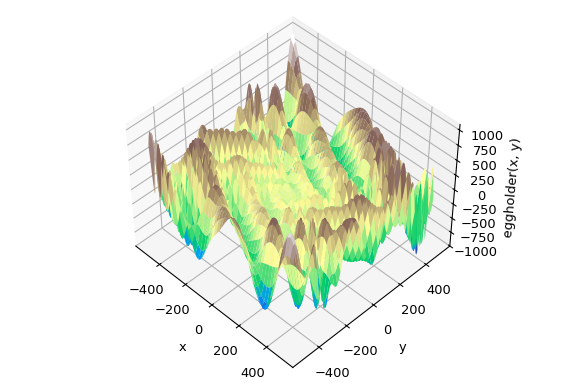
全局优化旨在给定边界内找到函数的全局最小值，即使存在许多局部最小值。通常，全局最小化器会有效地搜索参数空间，同时在底层使用局部最小化器（例如，minimize）。SciPy 包含许多优秀的全局优化器。在这里，我们将使用这些优化器处理相同的目标函数，即（恰当地命名的）eggholder 函数

>>> def eggholder(x):
...     return (-(x[1] + 47) * np.sin(np.sqrt(abs(x[0]/2 + (x[1]  + 47))))
...             -x[0] * np.sin(np.sqrt(abs(x[0] - (x[1]  + 47)))))

>>> bounds = [(-512, 512), (-512, 512)]

这个函数看起来像一个蛋托

>>> import matplotlib.pyplot as plt
>>> from mpl_toolkits.mplot3d import Axes3D

>>> x = np.arange(-512, 513)
>>> y = np.arange(-512, 513)
>>> xgrid, ygrid = np.meshgrid(x, y)
>>> xy = np.stack([xgrid, ygrid])

>>> fig = plt.figure()
>>> ax = fig.add_subplot(111, projection='3d')
>>> ax.view_init(45, -45)
>>> ax.plot_surface(xgrid, ygrid, eggholder(xy), cmap='terrain')
>>> ax.set_xlabel('x')
>>> ax.set_ylabel('y')
>>> ax.set_zlabel('eggholder(x, y)')
>>> plt.show()

我们现在使用全局优化器来获取最小值以及函数在最小值处的值。我们将结果存储在一个字典中，以便稍后比较不同的优化结果。

>>> from scipy import optimize
>>> results = dict()
>>> results['shgo'] = optimize.shgo(eggholder, bounds)
>>> results['shgo']
     fun: -935.3379515604197  # may vary
    funl: array([-935.33795156])
 message: 'Optimization terminated successfully.'
    nfev: 42
     nit: 2
   nlfev: 37
   nlhev: 0
   nljev: 9
 success: True
       x: array([439.48096952, 453.97740589])
      xl: array([[439.48096952, 453.97740589]])

>>> results['DA'] = optimize.dual_annealing(eggholder, bounds)
>>> results['DA']
     fun: -956.9182316237413  # may vary
 message: ['Maximum number of iteration reached']
    nfev: 4091
    nhev: 0
     nit: 1000
    njev: 0
       x: array([482.35324114, 432.87892901])

所有优化器都返回一个 OptimizeResult，除了解决方案之外，它还包含有关函数评估次数、优化是否成功等信息。为简洁起见，我们不会显示其他优化器的完整输出

>>> results['DE'] = optimize.differential_evolution(eggholder, bounds)

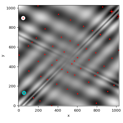
shgo 有第二种方法，它返回所有局部最小值，而不仅仅是它认为的全局最小值

>>> results['shgo_sobol'] = optimize.shgo(eggholder, bounds, n=200, iters=5,
...                                       sampling_method='sobol')

我们现在将在函数的热图上绘制所有找到的最小值

>>> fig = plt.figure()
>>> ax = fig.add_subplot(111)
>>> im = ax.imshow(eggholder(xy), interpolation='bilinear', origin='lower',
...                cmap='gray')
>>> ax.set_xlabel('x')
>>> ax.set_ylabel('y')
>>>
>>> def plot_point(res, marker='o', color=None):
...     ax.plot(512+res.x[0], 512+res.x[1], marker=marker, color=color, ms=10)

>>> plot_point(results['DE'], color='c')  # differential_evolution - cyan
>>> plot_point(results['DA'], color='w')  # dual_annealing.        - white

>>> # SHGO produces multiple minima, plot them all (with a smaller marker size)
>>> plot_point(results['shgo'], color='r', marker='+')
>>> plot_point(results['shgo_sobol'], color='r', marker='x')
>>> for i in range(results['shgo_sobol'].xl.shape[0]):
...     ax.plot(512 + results['shgo_sobol'].xl[i, 0],
...             512 + results['shgo_sobol'].xl[i, 1],
...             'ro', ms=2)

>>> ax.set_xlim([-4, 514*2])
>>> ax.set_ylim([-4, 514*2])
>>> plt.show()

全局优化器比较

使用下表查找满足您要求的求解器。如果有多个候选者，请尝试几个并查看哪个最能满足您的需求（例如，执行时间、目标函数值）。

求解器	边界约束	非线性约束	使用梯度	使用黑塞矩阵
basinhopping			(✓)	(✓)
direct	✓
dual_annealing	✓		(✓)	(✓)
differential_evolution	✓	✓
shgo	✓	✓	(✓)	(✓)

(✓) = 取决于选择的局部极小化器

最小二乘极小化 (least_squares)

SciPy 能够解决以下形式的鲁棒化边界约束非线性最小二乘问题

\begin{align} &\min_\mathbf{x} \frac{1}{2} \sum_{i = 1}^m \rho\left(f_i(\mathbf{x})^2\right) \\ &\text{subject to }\mathbf{lb} \leq \mathbf{x} \leq \mathbf{ub} \end{align}

其中 \(f_i(\mathbf{x})\) 是从 \(\mathbb{R}^n\) 到 \(\mathbb{R}\) 的平滑函数，我们称它们为残差。标量值函数 \(\rho(\cdot)\) 的目的是减少异常残差的影响，并有助于解的鲁棒性，我们称它为损失函数。线性损失函数给出了标准最小二乘问题。此外，允许对某些 \(x_j\) 设置下限和上限形式的约束。

所有特定于最小二乘极小化的方法都使用一个 \(m \times n\) 的偏导数矩阵，称为雅可比矩阵，定义为 \(J_{ij} = \partial f_i / \partial x_j\)。强烈建议分析计算此矩阵并将其传递给 least_squares，否则，它将通过有限差分进行估计，这会花费大量额外时间，并且在困难情况下可能非常不准确。

函数 least_squares 可用于将函数 \(\varphi(t; \mathbf{x})\) 拟合到经验数据 \(\{(t_i, y_i), i = 0, \ldots, m-1\}\)。为此，只需将残差预计算为 \(f_i(\mathbf{x}) = w_i (\varphi(t_i; \mathbf{x}) - y_i)\)，其中 \(w_i\) 是分配给每个观测值的权重。

求解拟合问题的示例

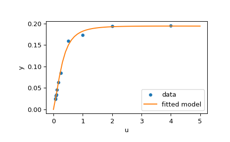
这里我们考虑一个酶促反应 [1]。有 11 个残差定义为

\[f_i(x) = \frac{x_0 (u_i^2 + u_i x_1)}{u_i^2 + u_i x_2 + x_3} - y_i, \quad i = 0, \ldots, 10,\]

其中 \(y_i\) 是测量值，\(u_i\) 是自变量的值。未知参数向量为 \(\mathbf{x} = (x_0, x_1, x_2, x_3)^T\)。如前所述，建议以封闭形式计算雅可比矩阵

\begin{align} &J_{i0} = \frac{\partial f_i}{\partial x_0} = \frac{u_i^2 + u_i x_1}{u_i^2 + u_i x_2 + x_3} \\ &J_{i1} = \frac{\partial f_i}{\partial x_1} = \frac{u_i x_0}{u_i^2 + u_i x_2 + x_3} \\ &J_{i2} = \frac{\partial f_i}{\partial x_2} = -\frac{x_0 (u_i^2 + u_i x_1) u_i}{(u_i^2 + u_i x_2 + x_3)^2} \\ &J_{i3} = \frac{\partial f_i}{\partial x_3} = -\frac{x_0 (u_i^2 + u_i x_1)}{(u_i^2 + u_i x_2 + x_3)^2} \end{align}

我们将使用 [2] 中定义的“硬”起始点。为了找到物理上有意义的解，避免潜在的除零错误并确保收敛到全局最小值，我们施加了约束 \(0 \leq x_j \leq 100, j = 0, 1, 2, 3\)。

下面的代码实现了 \(\mathbf{x}\) 的最小二乘估计，最后绘制了原始数据和拟合的模型函数

>>> from scipy.optimize import least_squares

>>> def model(x, u):
...     return x[0] * (u ** 2 + x[1] * u) / (u ** 2 + x[2] * u + x[3])

>>> def fun(x, u, y):
...     return model(x, u) - y

>>> def jac(x, u, y):
...     J = np.empty((u.size, x.size))
...     den = u ** 2 + x[2] * u + x[3]
...     num = u ** 2 + x[1] * u
...     J[:, 0] = num / den
...     J[:, 1] = x[0] * u / den
...     J[:, 2] = -x[0] * num * u / den ** 2
...     J[:, 3] = -x[0] * num / den ** 2
...     return J

>>> u = np.array([4.0, 2.0, 1.0, 5.0e-1, 2.5e-1, 1.67e-1, 1.25e-1, 1.0e-1,
...               8.33e-2, 7.14e-2, 6.25e-2])
>>> y = np.array([1.957e-1, 1.947e-1, 1.735e-1, 1.6e-1, 8.44e-2, 6.27e-2,
...               4.56e-2, 3.42e-2, 3.23e-2, 2.35e-2, 2.46e-2])
>>> x0 = np.array([2.5, 3.9, 4.15, 3.9])
>>> res = least_squares(fun, x0, jac=jac, bounds=(0, 100), args=(u, y), verbose=1)
# may vary
`ftol` termination condition is satisfied.
Function evaluations 130, initial cost 4.4383e+00, final cost 1.5375e-04, first-order optimality 4.92e-08.
>>> res.x
array([ 0.19280596,  0.19130423,  0.12306063,  0.13607247])

>>> import matplotlib.pyplot as plt
>>> u_test = np.linspace(0, 5)
>>> y_test = model(res.x, u_test)
>>> plt.plot(u, y, 'o', markersize=4, label='data')
>>> plt.plot(u_test, y_test, label='fitted model')
>>> plt.xlabel("u")
>>> plt.ylabel("y")
>>> plt.legend(loc='lower right')
>>> plt.show()

[1]

J. Kowalik and J. F. Morrison, "别构酶反应动力学数据的非线性回归问题分析", Math. Biosci., vol. 2, pp. 57-66, 1968.

[2]

2. 13. Averick et al., "MINPACK-2 测试问题集".

更多示例

下面的三个交互式示例更详细地说明了 least_squares 的用法。

1. scipy 中的大规模束调整 演示了 least_squares 的大规模功能以及如何高效计算稀疏雅可比矩阵的有限差分近似。

2. scipy 中的鲁棒非线性回归 展示了如何在非线性回归中使用鲁棒损失函数处理异常值。

3. scipy 中求解离散边值问题 研究了如何求解大型方程组并使用边界来获得所需的解性质。

有关实现背后的数学算法的详细信息，请参阅 least_squares 的文档。

一元函数极小化器 (minimize_scalar)

通常只需要一元函数（即，接受标量作为输入的函数）的最小值。在这种情况下，已经开发出其他可以更快工作的优化技术。这些可以通过 minimize_scalar 函数访问，该函数提供了几种算法。

无约束极小化 (method='brent')

实际上，有两种方法可以用于极小化一元函数：brent 和 golden，但 golden 仅用于学术目的，很少使用。这些方法分别可以通过 minimize_scalar 中的 method 参数选择。brent 方法使用 Brent 算法定位最小值。理想情况下，应提供一个包含所需最小值的区间（bracket 参数）。区间是一个三元组 \(\left( a, b, c \right)\)，使得 \(f \left( a \right) > f \left( b \right) < f \left( c \right)\) 且 \(a < b < c\)。如果未提供此参数，则可以选择两个起始点，然后使用简单的行进算法从这些点找到一个区间。如果未提供这两个起始点，将使用 0 和 1（这可能不是您函数正确的选择，并导致返回意外的最小值）。

这是一个例子

>>> from scipy.optimize import minimize_scalar
>>> f = lambda x: (x - 2) * (x + 1)**2
>>> res = minimize_scalar(f, method='brent')
>>> print(res.x)
1.0

有界极小化 (method='bounded')

通常，在进行极小化之前，可以对解空间施加约束。minimize_scalar 中的 bounded 方法是约束极小化过程的一个示例，它为标量函数提供了基本的区间约束。区间约束允许极小化仅发生在两个固定端点之间，使用强制性的 bounds 参数指定。

例如，为了找到 \(J_{1}\left( x \right)\) 在 \(x=5\) 附近的最小值，可以使用区间 \(\left[ 4, 7 \right]\) 作为约束来调用 minimize_scalar。结果是 \(x_{\textrm{min}}=5.3314\)

>>> from scipy.special import j1
>>> res = minimize_scalar(j1, bounds=(4, 7), method='bounded')
>>> res.x
5.33144184241

自定义极小化器

有时，使用自定义方法作为（多元或一元）极小化器可能很有用，例如，在使用某些 minimize 的库包装器（例如 basinhopping）时。

我们可以通过传递可调用对象（函数或实现了 __call__ 方法的对象）作为 method 参数来实现这一点，而不是传递方法名称。

让我们考虑一个（ admittedly rather virtual）需要使用一个简单的自定义多元极小化方法，该方法将以固定步长独立搜索每个维度的邻域

>>> from scipy.optimize import OptimizeResult
>>> def custmin(fun, x0, args=(), maxfev=None, stepsize=0.1,
...         maxiter=100, callback=None, **options):
...     bestx = x0
...     besty = fun(x0)
...     funcalls = 1
...     niter = 0
...     improved = True
...     stop = False
...
...     while improved and not stop and niter < maxiter:
...         improved = False
...         niter += 1
...         for dim in range(np.size(x0)):
...             for s in [bestx[dim] - stepsize, bestx[dim] + stepsize]:
...                 testx = np.copy(bestx)
...                 testx[dim] = s
...                 testy = fun(testx, *args)
...                 funcalls += 1
...                 if testy < besty:
...                     besty = testy
...                     bestx = testx
...                     improved = True
...             if callback is not None:
...                 callback(bestx)
...             if maxfev is not None and funcalls >= maxfev:
...                 stop = True
...                 break
...
...     return OptimizeResult(fun=besty, x=bestx, nit=niter,
...                           nfev=funcalls, success=(niter > 1))
>>> x0 = [1.35, 0.9, 0.8, 1.1, 1.2]
>>> res = minimize(rosen, x0, method=custmin, options=dict(stepsize=0.05))
>>> res.x
array([1., 1., 1., 1., 1.])

这在一元优化中也同样有效

>>> def custmin(fun, bracket, args=(), maxfev=None, stepsize=0.1,
...         maxiter=100, callback=None, **options):
...     bestx = (bracket[1] + bracket[0]) / 2.0
...     besty = fun(bestx)
...     funcalls = 1
...     niter = 0
...     improved = True
...     stop = False
...
...     while improved and not stop and niter < maxiter:
...         improved = False
...         niter += 1
...         for testx in [bestx - stepsize, bestx + stepsize]:
...             testy = fun(testx, *args)
...             funcalls += 1
...             if testy < besty:
...                 besty = testy
...                 bestx = testx
...                 improved = True
...         if callback is not None:
...             callback(bestx)
...         if maxfev is not None and funcalls >= maxfev:
...             stop = True
...             break
...
...     return OptimizeResult(fun=besty, x=bestx, nit=niter,
...                           nfev=funcalls, success=(niter > 1))
>>> def f(x):
...    return (x - 2)**2 * (x + 2)**2
>>> res = minimize_scalar(f, bracket=(-3.5, 0), method=custmin,
...                       options=dict(stepsize = 0.05))
>>> res.x
-2.0

求根

标量函数

如果有一个单变量方程，可以尝试多种不同的求根算法。这些算法中的大多数都需要一个根预期存在的区间的端点（因为函数会改变符号）。通常，brentq 是最佳选择，但其他方法在某些情况下或出于学术目的可能有用。当区间不可用，但有一个或多个导数可用时，newton（或 halley，secant）可能适用。当函数定义在复平面的子集上，并且无法使用区间方法时，尤其如此。

不动点求解

与求函数零点密切相关的问题是求函数不动点的问题。函数的不动点是函数求值后返回该点的点：\(g\left(x\right)=x.\) 显然，\(g\) 的不动点是 \(f\left(x\right)=g\left(x\right)-x.\) 的根。同样，\(f\) 的根是 \(g\left(x\right)=f\left(x\right)+x.\) 的不动点。fixed_point 例程提供了一种简单的迭代方法，使用 Aitkens 序列加速来估计给定起始点 \(g\) 的不动点。

方程组

可以使用 root 函数求解一组非线性方程的根。有几种方法可用，其中包括 hybr（默认）和 lm，它们分别使用 Powell 的混合方法和 MINPACK 的 Levenberg-Marquardt 方法。

下面的例子考虑了单变量超越方程

\[x+2\cos\left(x\right)=0,\]

其根可以按如下方式找到

>>> import numpy as np
>>> from scipy.optimize import root
>>> def func(x):
...     return x + 2 * np.cos(x)
>>> sol = root(func, 0.3)
>>> sol.x
array([-1.02986653])
>>> sol.fun
array([ -6.66133815e-16])

现在考虑一组非线性方程

\begin{eqnarray*} x_{0}\cos\left(x_{1}\right) & = & 4,\\ x_{0}x_{1}-x_{1} & = & 5. \end{eqnarray*}

我们定义目标函数，使其也返回雅可比矩阵，并通过将 jac 参数设置为 True 来指示这一点。此外，这里使用了 Levenberg-Marquardt 求解器。

>>> def func2(x):
...     f = [x[0] * np.cos(x[1]) - 4,
...          x[1]*x[0] - x[1] - 5]
...     df = np.array([[np.cos(x[1]), -x[0] * np.sin(x[1])],
...                    [x[1], x[0] - 1]])
...     return f, df
>>> sol = root(func2, [1, 1], jac=True, method='lm')
>>> sol.x
array([ 6.50409711,  0.90841421])

大型问题的求根

root 中的 hybr 和 lm 方法无法处理大量的变量 (N)，因为它们需要在每个牛顿步中计算和反转一个稠密的 N x N 雅可比矩阵。当 N 增大时，这会变得相当低效。

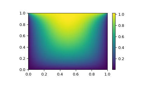
例如，考虑以下问题：我们需要在正方形 \([0,1]\times[0,1]\) 上求解以下积分微分方程

\[(\partial_x^2 + \partial_y^2) P + 5 \left(\int_0^1\int_0^1\cosh(P)\,dx\,dy\right)^2 = 0\]

边界条件为上边缘 \(P(x,1) = 1\)，正方形边界其他地方为 \(P=0\)。这可以通过将连续函数 P 近似为其在网格上的值，即 \(P_{n,m}\approx{}P(n h, m h)\)，其中网格间距 h 较小。然后可以近似导数和积分；例如 \(\partial_x^2 P(x,y)\approx{}(P(x+h,y) - 2 P(x,y) + P(x-h,y))/h^2\)。然后，该问题等同于寻找某个函数 residual(P) 的根，其中 P 是长度为 \(N_x N_y\) 的向量。

现在，由于 \(N_x N_y\) 可能很大，root 中的 hybr 或 lm 方法解决此问题将花费很长时间。然而，可以使用大型求解器之一来找到解决方案，例如 krylov、broyden2 或 anderson。这些方法使用所谓的非精确牛顿法，该方法不是精确计算雅可比矩阵，而是对其进行近似。

我们现在的问题可以通过以下方式解决

import numpy as np
from scipy.optimize import root
from numpy import cosh, zeros_like, mgrid, zeros

# parameters
nx, ny = 75, 75
hx, hy = 1./(nx-1), 1./(ny-1)

P_left, P_right = 0, 0
P_top, P_bottom = 1, 0

def residual(P):
   d2x = zeros_like(P)
   d2y = zeros_like(P)

   d2x[1:-1] = (P[2:]   - 2*P[1:-1] + P[:-2]) / hx/hx
   d2x[0]    = (P[1]    - 2*P[0]    + P_left)/hx/hx
   d2x[-1]   = (P_right - 2*P[-1]   + P[-2])/hx/hx

   d2y[:,1:-1] = (P[:,2:] - 2*P[:,1:-1] + P[:,:-2])/hy/hy
   d2y[:,0]    = (P[:,1]  - 2*P[:,0]    + P_bottom)/hy/hy
   d2y[:,-1]   = (P_top   - 2*P[:,-1]   + P[:,-2])/hy/hy

   return d2x + d2y + 5*cosh(P).mean()**2

# solve
guess = zeros((nx, ny), float)
sol = root(residual, guess, method='krylov', options={'disp': True})
#sol = root(residual, guess, method='broyden2', options={'disp': True, 'max_rank': 50})
#sol = root(residual, guess, method='anderson', options={'disp': True, 'M': 10})
print('Residual: %g' % abs(residual(sol.x)).max())

# visualize
import matplotlib.pyplot as plt
x, y = mgrid[0:1:(nx*1j), 0:1:(ny*1j)]
plt.pcolormesh(x, y, sol.x, shading='gouraud')
plt.colorbar()
plt.show()

仍然太慢？预处理。

当寻找函数 \(f_i({\bf x}) = 0\), i = 1, 2, …, N 的零点时，krylov 求解器大部分时间都在反转雅可比矩阵，

\[J_{ij} = \frac{\partial f_i}{\partial x_j} .\]

如果您有逆矩阵 \(M\approx{}J^{-1}\) 的近似值，则可以使用它对线性反演问题进行预处理。其思想是，不是求解 \(J{\bf s}={\bf y}\)，而是求解 \(MJ{\bf s}=M{\bf y}\)：由于矩阵 \(MJ\) 比 \(J\) “更接近”单位矩阵，因此 Krylov 方法应该更容易处理该方程。

矩阵 M 可以通过 krylov 方法的选项 options['jac_options']['inner_M'] 传递给 root。它可以是（稀疏）矩阵或 scipy.sparse.linalg.LinearOperator 实例。

对于上一节中的问题，我们注意到要解决的函数由两部分组成：第一部分是拉普拉斯算子的应用，\([\partial_x^2 + \partial_y^2] P\)，第二部分是积分。我们实际上可以很容易地计算出对应于拉普拉斯算子部分的雅可比矩阵：我们知道在一维中

\[\begin{split}\partial_x^2 \approx \frac{1}{h_x^2} \begin{pmatrix} -2 & 1 & 0 & 0 \cdots \\ 1 & -2 & 1 & 0 \cdots \\ 0 & 1 & -2 & 1 \cdots \\ \ldots \end{pmatrix} = h_x^{-2} L\end{split}\]

因此整个二维算子表示为

\[J_1 = \partial_x^2 + \partial_y^2 \simeq h_x^{-2} L \otimes I + h_y^{-2} I \otimes L\]

对应于积分的雅可比矩阵 \(J_2\) 更难计算，并且由于其所有项都非零，因此难以求逆。\(J_1\) 另一方面是一个相对简单的矩阵，可以通过 scipy.sparse.linalg.splu 求逆（或者可以通过 scipy.sparse.linalg.spilu 近似其逆）。所以我们满足于取 \(M\approx{}J_1^{-1}\) 并希望结果良好。

在下面的示例中，我们使用预处理器 \(M=J_1^{-1}\)。

from scipy.optimize import root
from scipy.sparse import dia_array, kron
from scipy.sparse.linalg import spilu, LinearOperator
from numpy import cosh, zeros_like, mgrid, zeros, eye

# parameters
nx, ny = 75, 75
hx, hy = 1./(nx-1), 1./(ny-1)

P_left, P_right = 0, 0
P_top, P_bottom = 1, 0

def get_preconditioner():
    """Compute the preconditioner M"""
    diags_x = zeros((3, nx))
    diags_x[0,:] = 1/hx/hx
    diags_x[1,:] = -2/hx/hx
    diags_x[2,:] = 1/hx/hx
    Lx = dia_array((diags_x, [-1,0,1]), shape=(nx, nx))

    diags_y = zeros((3, ny))
    diags_y[0,:] = 1/hy/hy
    diags_y[1,:] = -2/hy/hy
    diags_y[2,:] = 1/hy/hy
    Ly = dia_array((diags_y, [-1,0,1]), shape=(ny, ny))

    J1 = kron(Lx, eye(ny)) + kron(eye(nx), Ly)

    # Now we have the matrix `J_1`. We need to find its inverse `M` --
    # however, since an approximate inverse is enough, we can use
    # the *incomplete LU* decomposition

    J1_ilu = spilu(J1)

    # This returns an object with a method .solve() that evaluates
    # the corresponding matrix-vector product. We need to wrap it into
    # a LinearOperator before it can be passed to the Krylov methods:

    M = LinearOperator(shape=(nx*ny, nx*ny), matvec=J1_ilu.solve)
    return M

def solve(preconditioning=True):
    """Compute the solution"""
    count = [0]

    def residual(P):
        count[0] += 1

        d2x = zeros_like(P)
        d2y = zeros_like(P)

        d2x[1:-1] = (P[2:]   - 2*P[1:-1] + P[:-2])/hx/hx
        d2x[0]    = (P[1]    - 2*P[0]    + P_left)/hx/hx
        d2x[-1]   = (P_right - 2*P[-1]   + P[-2])/hx/hx

        d2y[:,1:-1] = (P[:,2:] - 2*P[:,1:-1] + P[:,:-2])/hy/hy
        d2y[:,0]    = (P[:,1]  - 2*P[:,0]    + P_bottom)/hy/hy
        d2y[:,-1]   = (P_top   - 2*P[:,-1]   + P[:,-2])/hy/hy

        return d2x + d2y + 5*cosh(P).mean()**2

    # preconditioner
    if preconditioning:
        M = get_preconditioner()
    else:
        M = None

    # solve
    guess = zeros((nx, ny), float)

    sol = root(residual, guess, method='krylov',
               options={'disp': True,
                        'jac_options': {'inner_M': M}})
    print('Residual', abs(residual(sol.x)).max())
    print('Evaluations', count[0])

    return sol.x

def main():
    sol = solve(preconditioning=True)

    # visualize
    import matplotlib.pyplot as plt
    x, y = mgrid[0:1:(nx*1j), 0:1:(ny*1j)]
    plt.clf()
    plt.pcolor(x, y, sol)
    plt.clim(0, 1)
    plt.colorbar()
    plt.show()


if __name__ == "__main__":
    main()

运行结果，首先不带预处理

0:  |F(x)| = 803.614; step 1; tol 0.000257947
1:  |F(x)| = 345.912; step 1; tol 0.166755
2:  |F(x)| = 139.159; step 1; tol 0.145657
3:  |F(x)| = 27.3682; step 1; tol 0.0348109
4:  |F(x)| = 1.03303; step 1; tol 0.00128227
5:  |F(x)| = 0.0406634; step 1; tol 0.00139451
6:  |F(x)| = 0.00344341; step 1; tol 0.00645373
7:  |F(x)| = 0.000153671; step 1; tol 0.00179246
8:  |F(x)| = 6.7424e-06; step 1; tol 0.00173256
Residual 3.57078908664e-07
Evaluations 317

然后带预处理

0:  |F(x)| = 136.993; step 1; tol 7.49599e-06
1:  |F(x)| = 4.80983; step 1; tol 0.00110945
2:  |F(x)| = 0.195942; step 1; tol 0.00149362
3:  |F(x)| = 0.000563597; step 1; tol 7.44604e-06
4:  |F(x)| = 1.00698e-09; step 1; tol 2.87308e-12
Residual 9.29603061195e-11
Evaluations 77

使用预处理器将 residual 函数的评估次数减少了 4 倍。对于计算残差成本高昂的问题，良好的预处理至关重要——它甚至可以决定问题在实践中是否可解。

预处理是一门艺术、一门科学，也是一个行业。在这里，我们很幸运做出了一个简单但效果不错的选择，但这个话题的深度远不止于此。

线性规划 (linprog)

函数 linprog 可以极小化受线性等式和不等式约束的线性目标函数。这类问题通常称为线性规划。线性规划解决以下形式的问题

\[\begin{split}\min_x \ & c^T x \\ \mbox{such that} \ & A_{ub} x \leq b_{ub},\\ & A_{eq} x = b_{eq},\\ & l \leq x \leq u ,\end{split}\]

其中 \(x\) 是决策变量向量；\(c\)、\(b_{ub}\)、\(b_{eq}\)、\(l\) 和 \(u\) 是向量；\(A_{ub}\) 和 \(A_{eq}\) 是矩阵。

在本教程中，我们将尝试使用 linprog 解决一个典型的线性规划问题。

线性规划示例

考虑以下简单的线性规划问题

\[\begin{split}\max_{x_1, x_2, x_3, x_4} \ & 29x_1 + 45x_2 \\ \mbox{such that} \ & x_1 -x_2 -3x_3 \leq 5\\ & 2x_1 -3x_2 -7x_3 + 3x_4 \geq 10\\ & 2x_1 + 8x_2 + x_3 = 60\\ & 4x_1 + 4x_2 + x_4 = 60\\ & 0 \leq x_0\\ & 0 \leq x_1 \leq 5\\ & x_2 \leq 0.5\\ & -3 \leq x_3\\\end{split}\]

我们需要一些数学操作来将目标问题转换为 linprog 接受的形式。

首先，让我们考虑目标函数。我们想最大化目标函数，但 linprog 只能接受最小化问题。这很容易通过将最大化 \(29x_1 + 45x_2\) 转换为最小化 \(-29x_1 -45x_2\) 来解决。此外，\(x_3, x_4\) 未显示在目标函数中。这意味着 \(x_3, x_4\) 对应的权重为零。因此，目标函数可以转换为

\[\min_{x_1, x_2, x_3, x_4} \ -29x_1 -45x_2 + 0x_3 + 0x_4\]

如果我们定义决策变量向量 \(x = [x_1, x_2, x_3, x_4]^T\)，则此问题中 linprog 的目标权重向量 \(c\) 应为

\[c = [-29, -45, 0, 0]^T\]

接下来，我们考虑两个不等式约束。第一个是“小于等于”不等式，因此它已经符合 linprog 接受的形式。第二个是“大于等于”不等式，因此我们需要将两边乘以 \(-1\) 将其转换为“小于等于”不等式。明确显示零系数，我们得到

\[\begin{split}x_1 -x_2 -3x_3 + 0x_4 &\leq 5\\ -2x_1 + 3x_2 + 7x_3 - 3x_4 &\leq -10\\\end{split}\]

这些方程可以转换为矩阵形式

\[\begin{split}A_{ub} x \leq b_{ub}\\\end{split}\]

其中

\begin{equation*} A_{ub} = \begin{bmatrix} 1 & -1 & -3 & 0 \\ -2 & 3 & 7 & -3 \end{bmatrix} \end{equation*}

\begin{equation*} b_{ub} = \begin{bmatrix} 5 \\ -10 \end{bmatrix} \end{equation*}

接下来，我们考虑两个等式约束。明确显示零权重，它们是

\[\begin{split}2x_1 + 8x_2 + 1x_3 + 0x_4 &= 60\\ 4x_1 + 4x_2 + 0x_3 + 1x_4 &= 60\\\end{split}\]

这些方程可以转换为矩阵形式

\[\begin{split}A_{eq} x = b_{eq}\\\end{split}\]

其中

\begin{equation*} A_{eq} = \begin{bmatrix} 2 & 8 & 1 & 0 \\ 4 & 4 & 0 & 1 \end{bmatrix} \end{equation*}

\begin{equation*} b_{eq} = \begin{bmatrix} 60 \\ 60 \end{bmatrix} \end{equation*}

最后，我们来考虑针对单个决策变量的独立不等式约束，这些约束被称为“盒约束”或“简单界限”。这些约束可以通过 linprog 函数的 bounds 参数应用。如 linprog 文档中所述，bounds 的默认值为 (0, None)，这意味着每个决策变量的下限为0，上限为无穷大：所有决策变量都是非负的。我们的界限不同，因此我们需要将每个决策变量的下限和上限指定为元组，并将这些元组组合成一个列表。

最后，我们可以使用 linprog 求解变换后的问题。

>>> import numpy as np
>>> from scipy.optimize import linprog
>>> c = np.array([-29.0, -45.0, 0.0, 0.0])
>>> A_ub = np.array([[1.0, -1.0, -3.0, 0.0],
...                 [-2.0, 3.0, 7.0, -3.0]])
>>> b_ub = np.array([5.0, -10.0])
>>> A_eq = np.array([[2.0, 8.0, 1.0, 0.0],
...                 [4.0, 4.0, 0.0, 1.0]])
>>> b_eq = np.array([60.0, 60.0])
>>> x0_bounds = (0, None)
>>> x1_bounds = (0, 5.0)
>>> x2_bounds = (-np.inf, 0.5)  # +/- np.inf can be used instead of None
>>> x3_bounds = (-3.0, None)
>>> bounds = [x0_bounds, x1_bounds, x2_bounds, x3_bounds]
>>> result = linprog(c, A_ub=A_ub, b_ub=b_ub, A_eq=A_eq, b_eq=b_eq, bounds=bounds)
>>> print(result.message)
The problem is infeasible. (HiGHS Status 8: model_status is Infeasible; primal_status is None)

结果表明我们的问题是不可行的，这意味着没有满足所有约束的解向量。这不一定意味着我们做错了什么；有些问题确实是不可行的。然而，假设我们决定对 \(x_1\) 的界限约束过紧，可以将其放宽至 \(0 \leq x_1 \leq 6\)。调整代码 x1_bounds = (0, 6) 以反映这一变化并再次执行后

>>> x1_bounds = (0, 6)
>>> bounds = [x0_bounds, x1_bounds, x2_bounds, x3_bounds]
>>> result = linprog(c, A_ub=A_ub, b_ub=b_ub, A_eq=A_eq, b_eq=b_eq, bounds=bounds)
>>> print(result.message)
Optimization terminated successfully. (HiGHS Status 7: Optimal)

结果表明优化成功。我们可以检查目标值（result.fun）是否与 \(c^Tx\) 相同

>>> x = np.array(result.x)
>>> obj = result.fun
>>> print(c @ x)
-505.97435889013434  # may vary
>>> print(obj)
-505.97435889013434  # may vary

我们还可以检查所有约束在合理容差范围内得到满足。

>>> print(b_ub - (A_ub @ x).flatten())  # this is equivalent to result.slack
[ 6.52747190e-10, -2.26730279e-09]  # may vary
>>> print(b_eq - (A_eq @ x).flatten())  # this is equivalent to result.con
[ 9.78840831e-09, 1.04662945e-08]]  # may vary
>>> print([0 <= result.x[0], 0 <= result.x[1] <= 6.0, result.x[2] <= 0.5, -3.0 <= result.x[3]])
[True, True, True, True]

分配问题

线性总和分配问题示例

考虑为游泳混合接力队选择学生的问题。我们有一张表，显示了五名学生每种泳姿的时间

学生	仰泳	蛙泳	蝶泳	自由泳
A	43.5	47.1	48.4	38.2
B	45.5	42.1	49.6	36.8
C	43.4	39.1	42.1	43.2
D	46.5	44.1	44.5	41.2
E	46.3	47.8	50.4	37.2

我们需要为四种泳姿各选择一名学生，以使总接力时间最短。这是一个典型的线性总和分配问题。我们可以使用 linear_sum_assignment 来解决它。

线性总和分配问题是最著名的组合优化问题之一。给定一个“成本矩阵” \(C\)，问题是选择

• 每行中恰好一个元素

• 不从任何列中选择超过一个元素

• 以使所选元素的总和最小化

换句话说，我们需要将每一行分配给一列，以使相应条目的总和最小化。

形式上，设 \(X\) 是一个布尔矩阵，当且仅当行 \(i\) 分配给列 \(j\) 时，\(X[i,j] = 1\)。则最优分配的成本为

\[\min \sum_i \sum_j C_{i,j} X_{i,j}\]

第一步是定义成本矩阵。在此示例中，我们希望将每种泳姿分配给一名学生。linear_sum_assignment 能够将成本矩阵的每一行分配给一列。因此，为了形成成本矩阵，上表需要转置，使得行对应泳姿，列对应学生

>>> import numpy as np
>>> cost = np.array([[43.5, 45.5, 43.4, 46.5, 46.3],
...                  [47.1, 42.1, 39.1, 44.1, 47.8],
...                  [48.4, 49.6, 42.1, 44.5, 50.4],
...                  [38.2, 36.8, 43.2, 41.2, 37.2]])

我们可以使用 linear_sum_assignment 解决分配问题

>>> from scipy.optimize import linear_sum_assignment
>>> row_ind, col_ind = linear_sum_assignment(cost)

row_ind 和 col_ind 是成本矩阵的最优分配矩阵索引

>>> row_ind
array([0, 1, 2, 3])
>>> col_ind
array([0, 2, 3, 1])

最优分配为

>>> styles = np.array(["backstroke", "breaststroke", "butterfly", "freestyle"])[row_ind]
>>> students = np.array(["A", "B", "C", "D", "E"])[col_ind]
>>> dict(zip(styles, students))
{'backstroke': 'A', 'breaststroke': 'C', 'butterfly': 'D', 'freestyle': 'B'}

最优总混合时间为

>>> cost[row_ind, col_ind].sum()
163.89999999999998

请注意，这个结果与每种泳姿的最小时间总和不同

>>> np.min(cost, axis=1).sum()
161.39999999999998

因为学生“C”在“蛙泳”和“蝶泳”方面都是最好的游泳者。我们不能将学生“C”分配给两种泳姿，因此我们将学生C分配给“蛙泳”，将学生D分配给“蝶泳”，以使总时间最小。

参考文献

一些进一步的阅读材料和相关软件，例如 Newton-Krylov [KK]、PETSc [PP] 和 PyAMG [AMG]

[KK]

D.A. Knoll and D.E. Keyes, “Jacobian-free Newton-Krylov methods”, J. Comp. Phys. 193, 357 (2004). DOI:10.1016/j.jcp.2003.08.010

[PP]

PETSc https://www.mcs.anl.gov/petsc/ and its Python bindings https://bitbucket.org/petsc/petsc4py/

[AMG]

PyAMG（代数多重网格预处理器/求解器） pyamg/pyamg#issues

混合整数线性规划

背包问题示例

背包问题是一个著名的组合优化问题。给定一组物品，每件物品都有一个大小和一个价值，问题是选择物品，使得在总大小低于某个阈值的条件下，总价值最大化。

形式上，设

• \(x_i\) 是一个布尔变量，表示物品 \(i\) 是否包含在背包中，

• \(n\) 是物品总数，

• \(v_i\) 是物品 \(i\) 的价值，

• \(s_i\) 是物品 \(i\) 的大小，并且

• \(C\) 是背包的容量。

则问题是

\[\max \sum_i^n v_{i} x_{i}\]

\[\text{subject to} \sum_i^n s_{i} x_{i} \leq C, x_{i} \in {0, 1}\]

尽管目标函数和不等式约束对于*决策变量* \(x_i\) 来说是线性的，但这与典型的线性规划问题不同，因为决策变量只能取整数值。具体来说，我们的决策变量只能是 \(0\) 或 \(1\)，因此这被称为*二进制整数线性规划* (BILP)。这样的问题属于更大一类的*混合整数线性规划* (MILPs)，我们可以使用 milp 来解决。

在我们的示例中，有8个物品可供选择，每个物品的大小和价值规定如下。

>>> import numpy as np
>>> from scipy import optimize
>>> sizes = np.array([21, 11, 15, 9, 34, 25, 41, 52])
>>> values = np.array([22, 12, 16, 10, 35, 26, 42, 53])

我们需要将八个决策变量约束为二进制。我们通过添加一个 Bounds 约束来确保它们介于 \(0\) 和 \(1\) 之间，并应用“整数性”约束以确保它们*是* \(0\) *或* \(1\)。

>>> bounds = optimize.Bounds(0, 1)  # 0 <= x_i <= 1
>>> integrality = np.full_like(values, True)  # x_i are integers

背包容量约束使用 LinearConstraint 指定。

>>> capacity = 100
>>> constraints = optimize.LinearConstraint(A=sizes, lb=0, ub=capacity)

如果我们遵循线性代数的常规规则，输入 A 应该是一个二维矩阵，下限 lb 和上限 ub 应该是一维向量，但只要输入可以广播到一致的形状，LinearConstraint 就能接受。

使用上面定义的变量，我们可以使用 milp 解决背包问题。请注意，milp 最小化目标函数，但我们希望最大化总价值，因此我们将 c 设置为价值的负值。

>>> from scipy.optimize import milp
>>> res = milp(c=-values, constraints=constraints,
...            integrality=integrality, bounds=bounds)

让我们检查结果

>>> res.success
True
>>> res.x
array([1., 1., 0., 1., 1., 1., 0., 0.])

这意味着我们应该选择物品1、2、4、5、6，以在尺寸约束下优化总价值。请注意，这与我们通过求解*线性规划松弛*（没有整数性约束）并尝试对决策变量进行四舍五入所得到的结果不同。

>>> from scipy.optimize import milp
>>> res = milp(c=-values, constraints=constraints,
...            integrality=False, bounds=bounds)
>>> res.x
array([1.        , 1.        , 1.        , 1.        ,
       0.55882353, 1.        , 0.        , 0.        ])

如果我们将这个解向上取整到 array([1., 1., 1., 1., 1., 1., 0., 0.])，我们的背包将超过容量约束，而如果向下取整到 array([1., 1., 1., 1., 0., 1., 0., 0.])，我们将得到一个次优解。

更多MILP教程，请参阅SciPy Cookbooks上的Jupyter notebooks。

• 压缩感知 l1 程序

• 压缩感知 l0 程序

并行执行支持

某些 SciPy 优化方法，例如 differential_evolution，通过使用 workers 关键字提供并行化支持。

对于 differential_evolution，算法中有两个循环（迭代）级别。外层循环表示种群的连续代。这个循环无法并行化。对于给定的代，会生成候选解，这些解必须与现有种群成员进行比较。候选解的适应度可以在循环中计算，但也可以并行化计算。

其他优化算法也可能实现并行化。例如，在各种 minimize 方法中，数值微分用于估计导数。对于使用两点前向差分的简单梯度计算，总共需要进行 N + 1 次目标函数计算，其中 N 是参数的数量。这些只是给定位置周围的微小扰动（即 +1 部分）。这 N + 1 次计算也可以并行化。最小化算法使用数值导数的计算来生成新步骤。

每种优化算法的工作方式都大相径庭，但它们通常在算法执行其他操作之前需要进行多次目标函数计算。这些位置就是可以并行化的地方。因此，workers 的使用方式存在一些共同特征。这些共同点如下所述。

如果提供一个整数，则会创建一个 multiprocessing.Pool 对象，并使用其 map 方法并行评估解决方案。采用这种方法，目标函数必须是可序列化的（pickleable）。Lambda 函数不满足该要求。

>>> import numpy as np
>>> from scipy.optimize import rosen, differential_evolution, Bounds
>>> bnds = Bounds([0., 0., 0.], [10., 10., 10.])
>>> res = differential_evolution(rosen, bnds, workers=2, updating='deferred')

也可以使用类似映射的可调用对象作为 worker。在这里，优化算法提供一系列向量，然后将这些向量提供给类似映射的函数。类似映射的函数需要根据目标函数评估每个向量。在以下示例中，我们使用 multiprocessing.Pool 作为类似映射的对象。和以前一样，目标函数仍然需要是可序列化的。这个例子在语义上与上一个例子相同。

>>> from multiprocessing import Pool
>>> with Pool(2) as pwl:
...     res = differential_evolution(rosen, bnds, workers=pwl.map, updating='deferred')

使用这种模式可能是一个优势，因为池可以重复用于进一步的计算——创建这些对象会产生大量的开销。multiprocessing.Pool 的替代方案包括 mpi4py 包，它可以在集群上实现并行处理。

在 Scipy 1.16.0 中，workers 关键字被引入到选定的 minimize 方法中。在这里，并行化通常应用于数值微分期间。上述两种方法都可以使用，但强烈建议提供类似映射的可调用对象，因为创建新进程会产生开销。只有当目标函数计算成本较高时，才能获得性能提升。让我们比较一下并行化与串行版本相比能带来多大帮助。为了模拟一个慢函数，我们使用 time 包。

>>> import time
>>> def slow_func(x):
...     time.sleep(0.0002)
...     return rosen(x)

首先检查串行最小化

In [1]: rng = np.random.default_rng()

In [2]: x0 = rng.uniform(low=0.0, high=10.0, size=(20,))

In [3]: %timeit minimize(slow_func, x0, method='L-BFGS-B')  # serial approach
365 ms ± 6.17 ms per loop (mean ± std. dev. of 7 runs, 1 loop each)  # may vary

现在是并行版本

In [4]: with Pool() as pwl:  # parallel approach
...         %timeit minimize(slow_func, x0, method='L-BFGS-B', options={'workers':pwl.map})
70.5 ms ± 146 μs per loop (mean ± std. dev. of 7 runs, 1 loop each)  # may vary

如果目标函数可以向量化，那么可以使用类似映射的对象在函数评估期间利用向量化。向量化意味着目标函数可以在单次（而非多次）调用中完成所需的计算，这通常非常高效

In [5]: def vectorized_maplike(fun, iterable):
...         arr = np.array([i for i in iter(iterable)])   # arr.shape = (S, N)
...         arr_t = arr.T                                 # arr_t.shape = (N, S)
...         r = slow_func(arr_t)                          # calculation vectorized over S
...         return r

In [6]: %timeit minimize(slow_func, x0, method='L-BFGS-B', options={'workers':vectorized_maplike})
38.9 ms ± 734 μs per loop (mean ± std. dev. of 7 runs, 10 loops each)  # may vary

关于这个示例，有几个重要的注意事项

• 可迭代对象表示算法希望评估的参数向量序列。

• 可迭代对象首先被转换为迭代器，然后通过列表推导式转换为数组。这使得可迭代对象可以是生成器、列表、数组等。

• 在类似映射的对象内部，计算是使用 slow_func 而不是 fun 来完成的。类似映射的对象实际上提供了目标函数的封装版本。封装用于检测各种常见的用户错误，包括检查目标函数是否返回标量。如果使用 fun，则会引发 RuntimeError，因为 fun(arr_t) 将是一个一维数组而不是标量。因此，我们直接使用 slow_func。

• arr.T 被发送到目标函数。这是因为 arr.shape == (S, N)，其中 S 是要评估的参数向量的数量，N 是变量的数量。对于 slow_func，向量化发生在 (N, S) 形状的数组上。

• 对于 differential_evolution，不需要这种方法，因为该最小化器已经有一个用于向量化的关键字。