scipy.signal.
dimpulse#
- scipy.signal.dimpulse(system, x0=None, t=None, n=None)[源码]#
离散时间系统的脉冲响应。
- 参数:
- systemdlti | 元组
LTI 类
dlti的实例,或描述系统的元组。元组中元素的数量决定了其解释方式。即:system: LTI 类dlti的实例。请注意,也允许使用派生实例,例如TransferFunction、ZerosPolesGain或StateSpace的实例。(num, den, dt): 如TransferFunction中所述的有理多项式。多项式的系数应按降幂顺序指定,例如,z² + 3z + 5 将表示为[1, 3, 5]。(zeros, poles, gain, dt): 如ZerosPolesGain中所述的零点、极点、增益形式。(A, B, C, D, dt): 如StateSpace中所述的状态空间形式。
- x0array_like, 可选
初始状态向量。默认为零。
- tarray_like, 可选
时间点。如果未给出,则计算。
- nint, 可选
要计算的时间点数量(如果未给出 t)。
- 返回:
- toutndarray
作为一维数组的输出时间值。
- youtndarray 元组
系统的脉冲响应。元组的每个元素表示系统基于每个输入的脉冲的输出。
另请参阅
示例
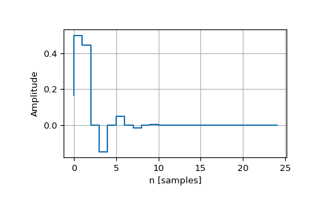
>>> import numpy as np
>>> from scipy import signal
>>> import matplotlib.pyplot as plt
...
>>> dt = 1  # sampling interval is one => time unit is sample number
>>> bb, aa = signal.butter(3, 0.25, fs=1/dt)
>>> t, y = signal.dimpulse((bb, aa, dt), n=25)
...
>>> fig0, ax0 = plt.subplots()
>>> ax0.step(t, np.squeeze(y), '.-', where='post')
>>> ax0.set_title(r"Impulse Response of a $3^\text{rd}$ Order Butterworth Filter")
>>> ax0.set(xlabel='Sample number', ylabel='Amplitude')
>>> ax0.grid()
>>> plt.show()