scipy.stats.genextreme

scipy.stats.genextreme = <scipy.stats._continuous_distns.genextreme_gen object>

广义极值连续随机变量。

作为 rv_continuous 类的实例，genextreme 对象从它继承了一组通用方法（请参阅下面的完整列表），并使用此特定分布的详细信息完成它们。

方法

rvs(c, loc=0, scale=1, size=1, random_state=None)	随机变量。
pdf(x, c, loc=0, scale=1)	概率密度函数。
logpdf(x, c, loc=0, scale=1)	概率密度函数的对数。
cdf(x, c, loc=0, scale=1)	累积分布函数。
logcdf(x, c, loc=0, scale=1)	累积分布函数的对数。
sf(x, c, loc=0, scale=1)	生存函数 (也定义为 1 - cdf, 但 sf 有时更准确).
logsf(x, c, loc=0, scale=1)	生存函数的对数。
ppf(q, c, loc=0, scale=1)	百分点函数 ( cdf 的逆函数 - 百分位数).
isf(q, c, loc=0, scale=1)	逆生存函数 ( sf 的逆函数).
moment(order, c, loc=0, scale=1)	指定阶的非中心矩。
stats(c, loc=0, scale=1, moments=’mv’)	均值 ('m')、方差 ('v')、偏度 ('s') 和/或峰度 ('k')。
entropy(c, loc=0, scale=1)	RV 的（微分）熵。
fit(data)	通用数据的参数估计。 有关关键字参数的详细文档，请参见 scipy.stats.rv_continuous.fit。
expect(func, args=(c,), loc=0, scale=1, lb=None, ub=None, conditional=False, **kwds)	函数（一个参数）相对于分布的期望值。
median(c, loc=0, scale=1)	分布的中位数。
mean(c, loc=0, scale=1)	分布的均值。
var(c, loc=0, scale=1)	分布的方差。
std(c, loc=0, scale=1)	分布的标准差。
interval(confidence, c, loc=0, scale=1)	中位数周围具有相等面积的置信区间。

参见

gumbel_r

笔记

对于 \(c=0\), genextreme 等于 gumbel_r 且概率密度函数为

\[f(x) = \exp(-\exp(-x)) \exp(-x),\]

其中 \(-\infty < x < \infty\).

对于 \(c \ne 0\), genextreme 的概率密度函数是

\[f(x, c) = \exp(-(1-c x)^{1/c}) (1-c x)^{1/c-1},\]

其中 \(-\infty < x \le 1/c\) 如果 \(c > 0\) 且 \(1/c \le x < \infty\) 如果 \(c < 0\).

请注意，一些来源和软件包使用形状参数 \(c\) 的符号的相反约定。

genextreme 将 c 作为 \(c\) 的形状参数。

上面的概率密度以“标准化”形式定义。 要移动和/或缩放分布，请使用 loc 和 scale 参数。 具体而言，genextreme.pdf(x, c, loc, scale) 与 genextreme.pdf(y, c) / scale 完全等效，其中 y = (x - loc) / scale。 请注意，移动分布的位置不会使其成为“非中心”分布； 一些分布的非中心泛化在单独的类中可用。

示例

在您的浏览器中尝试一下！

>>> import numpy as np
>>> from scipy.stats import genextreme
>>> import matplotlib.pyplot as plt
>>> fig, ax = plt.subplots(1, 1)

获取支持

>>> c = -0.1
>>> lb, ub = genextreme.support(c)

计算前四个矩

>>> mean, var, skew, kurt = genextreme.stats(c, moments='mvsk')

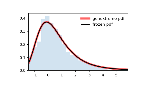
显示概率密度函数 (pdf)

>>> x = np.linspace(genextreme.ppf(0.01, c),
...                 genextreme.ppf(0.99, c), 100)
>>> ax.plot(x, genextreme.pdf(x, c),
...        'r-', lw=5, alpha=0.6, label='genextreme pdf')

或者，可以调用分布对象（作为函数）来固定形状、位置和比例参数。 这将返回一个“冻结”的 RV 对象，该对象保存给定的固定参数。

冻结分布并显示冻结的 pdf

>>> rv = genextreme(c)
>>> ax.plot(x, rv.pdf(x), 'k-', lw=2, label='frozen pdf')

检查 cdf 和 ppf 的准确性

>>> vals = genextreme.ppf([0.001, 0.5, 0.999], c)
>>> np.allclose([0.001, 0.5, 0.999], genextreme.cdf(vals, c))
True

生成随机数

>>> r = genextreme.rvs(c, size=1000)

并比较直方图

>>> ax.hist(r, density=True, bins='auto', histtype='stepfilled', alpha=0.2)
>>> ax.set_xlim([x[0], x[-1]])
>>> ax.legend(loc='best', frameon=False)
>>> plt.show()

返回在新标签页中打开