相干性#
- scipy.signal.coherence(x, y, fs=1.0, window='hann', nperseg=None, noverlap=None, nfft=None, detrend='constant', axis=-1)[source]#
使用Welch方法估计离散时间信号X和Y的幅度平方相干估计Cxy。
Cxy = abs(Pxy)**2/(Pxx*Pyy),其中 Pxx 和 Pyy 是 X 和 Y 的功率谱密度估计,Pxy 是 X 和 Y 的互谱密度估计。- 参数:
- xarray_like
测量值的时间序列
- yarray_like
测量值的时间序列
- fs浮点型,可选
x 和 y 时间序列的采样频率。默认为 1.0。
- window字符串、元组或类数组,可选
要使用的期望窗口。如果 window 是字符串或元组,则会将其传递给
get_window以生成窗口值,这些值默认为DFT偶数。有关窗口列表和所需参数,请参阅get_window。如果 window 是类数组,则将直接用作窗口,其长度必须为 nperseg。默认为汉宁窗口。- nperseg整型,可选
每个段的长度。默认为 None,但如果 window 是字符串或元组,则设置为 256;如果 window 是类数组,则设置为窗口的长度。
- noverlap: 整型,可选
段之间的重叠点数。如果为 None,则
noverlap = nperseg // 2。默认为 None。- nfft整型,可选
使用的FFT长度,如果需要零填充FFT。如果为 None,则FFT长度为 nperseg。默认为 None。
- detrend字符串、函数或布尔值False,可选
指定如何对每个段进行去趋势处理。如果
detrend是字符串,则将其作为 type 参数传递给detrend函数。如果它是一个函数,则接受一个段并返回一个去趋势处理后的段。如果detrend为 False,则不执行去趋势处理。默认为 'constant'。- axis整型,可选
用于计算两个输入的相干性的轴;默认为最后一个轴(即
axis=-1)。
- 返回:
- fndarray
采样频率数组。
- Cxyndarray
x 和 y 的幅度平方相干性。
另请参阅
periodogram简单,可选修改的周期图
lombscargle用于非均匀采样数据的Lomb-Scargle周期图
welch使用Welch方法计算的功率谱密度。
csd使用Welch方法计算的互谱密度。
备注
适当的重叠量将取决于窗口的选择和您的要求。对于默认的汉宁窗口,50% 的重叠是在准确估计信号功率和不过度统计任何数据之间的一个合理折衷。更窄的窗口可能需要更大的重叠。
在版本 0.16.0 中添加。
参考文献
[1]P. Welch, “The use of the fast Fourier transform for the estimation of power spectra: A method based on time averaging over short, modified periodograms”, IEEE Trans. Audio Electroacoust. vol. 15, pp. 70-73, 1967.
[2]Stoica, Petre, and Randolph Moses, “Spectral Analysis of Signals” Prentice Hall, 2005
示例
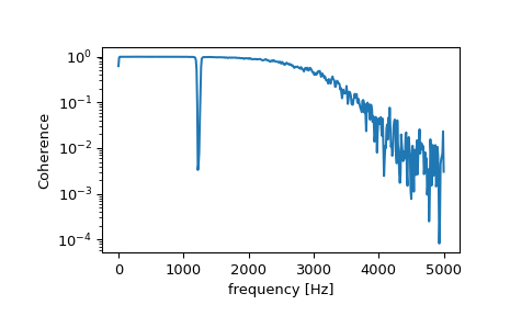
>>> import numpy as np
>>> from scipy import signal
>>> import matplotlib.pyplot as plt
>>> rng = np.random.default_rng()
生成两个具有一些共同特征的测试信号。
>>> fs = 10e3
>>> N = 1e5
>>> amp = 20
>>> freq = 1234.0
>>> noise_power = 0.001 * fs / 2
>>> time = np.arange(N) / fs
>>> b, a = signal.butter(2, 0.25, 'low')
>>> x = rng.normal(scale=np.sqrt(noise_power), size=time.shape)
>>> y = signal.lfilter(b, a, x)
>>> x += amp*np.sin(2*np.pi*freq*time)
>>> y += rng.normal(scale=0.1*np.sqrt(noise_power), size=time.shape)
计算并绘制相干性。
>>> f, Cxy = signal.coherence(x, y, fs, nperseg=1024)
>>> plt.semilogy(f, Cxy)
>>> plt.xlabel('frequency [Hz]')
>>> plt.ylabel('Coherence')
>>> plt.show()