外推技巧与窍门#
外推处理——在插值数据域外查询点上评估插值器——在 scipy.interpolate 的不同例程中并不完全一致。不同的插值器使用不同的关键字参数集来控制数据域之外的行为:有些使用 extrapolate=True/False/None,有些允许使用 fill_value 关键字。有关每个特定插值例程的详细信息,请参阅 API 文档。
根据特定问题,可用的关键字可能足够,也可能不足。需要特别注意非线性插值器的外推。通常,外推结果与数据域的距离越大,意义越小。这当然是意料之中的:插值器只知道数据域内的数据。
当默认的外推结果不充分时,用户需要自己实现所需的外推模式。
在本教程中,我们将考虑几个实际示例,演示可用关键字的使用以及所需外推模式的手动实现。这些示例可能适用于您的特定问题,也可能不适用;它们不一定是最佳实践;并且它们被特意简化为演示主要思想所需的基本要素,希望它们能为处理您的特定问题提供灵感。
interp1d : 复制 numpy.interp 的左右填充值#
TL;DR: 使用 fill_value=(left, right)
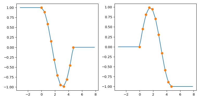
numpy.interp 使用常数外推,并默认将插值区间中 y 数组的第一个和最后一个值进行扩展:np.interp(xnew, x, y) 的输出对于 xnew < x[0] 是 y[0],对于 xnew > x[-1] 是 y[-1]。
默认情况下,interp1d 拒绝外推,当在插值范围之外的数据点上进行评估时,会引发 ValueError。这可以通过 bounds_error=False 参数关闭:此时 interp1d 使用 fill_value 设置超出范围的值,默认为 nan。
为了模仿 numpy.interp 与 interp1d 的行为,您可以利用它支持 2 元组作为 fill_value 的事实。元组元素将分别用于填充 xnew < min(x) 和 x > max(x)。对于多维 y,这些元素的形状必须与 y 相同或可广播到 y。
图示
import numpy as np
import matplotlib.pyplot as plt
from scipy.interpolate import interp1d

x = np.linspace(0, 1.5*np.pi, 11)
y = np.column_stack((np.cos(x), np.sin(x)))   # y.shape is (11, 2)

func = interp1d(x, y,
                axis=0,  # interpolate along columns
                bounds_error=False,
                kind='linear',
                fill_value=(y[0], y[-1]))
xnew = np.linspace(-np.pi, 2.5*np.pi, 51)
ynew = func(xnew)

fix, (ax1, ax2) = plt.subplots(1, 2, figsize=(8, 4))
ax1.plot(xnew, ynew[:, 0])
ax1.plot(x, y[:, 0], 'o')

ax2.plot(xnew, ynew[:, 1])
ax2.plot(x, y[:, 1], 'o')
plt.tight_layout()
CubicSpline 扩展边界条件#
CubicSpline 需要两个额外的边界条件,这些条件由 bc_type 参数控制。此参数可以列出边界处导数的显式值,也可以使用有用的别名。例如,bc_type="clamped" 将一阶导数设置为零,bc_type="natural" 将二阶导数设置为零(另外两个可识别的字符串值是“periodic”和“not-a-knot”)。
虽然外推由边界条件控制,但其关系并不十分直观。例如,人们可能期望对于 bc_type="natural",外推是线性的。这种期望过于强烈:每个边界条件只在边界上的一个点设置导数。外推是从第一个和最后一个多项式段进行的,对于自然样条来说,这是一个在给定点处二阶导数为零的三次多项式。
另一种说明这种期望为何过于强烈的方法是考虑一个只有三个数据点的数据集,其中样条有两个多项式段。为了线性外推,这种期望意味着这两个段都是线性的。但是,两个线性段不可能在中间点以连续的二阶导数匹配!(除非当然,所有三个数据点实际上都位于一条直线上)。
为了说明其行为,我们考虑一个合成数据集并比较几种边界条件
import numpy as np
import matplotlib.pyplot as plt
from scipy.interpolate import CubicSpline

xs = [1, 2, 3, 4, 5, 6, 7, 8]
ys = [4.5, 3.6, 1.6, 0.0, -3.3, -3.1, -1.8, -1.7]

notaknot = CubicSpline(xs, ys, bc_type='not-a-knot')
natural = CubicSpline(xs, ys, bc_type='natural')
clamped = CubicSpline(xs, ys, bc_type='clamped')
xnew = np.linspace(min(xs) - 4, max(xs) + 4, 101)

splines = [notaknot, natural, clamped]
titles = ['not-a-knot', 'natural', 'clamped']

fig, axs = plt.subplots(3, 3, figsize=(12, 12))
for i in [0, 1, 2]:
    for j, spline, title in zip(range(3), splines, titles):
        axs[i, j].plot(xs, spline(xs, nu=i),'o')
        axs[i, j].plot(xnew, spline(xnew, nu=i),'-')
        axs[i, j].set_title(f'{title}, deriv={i}')

plt.tight_layout()
plt.show()
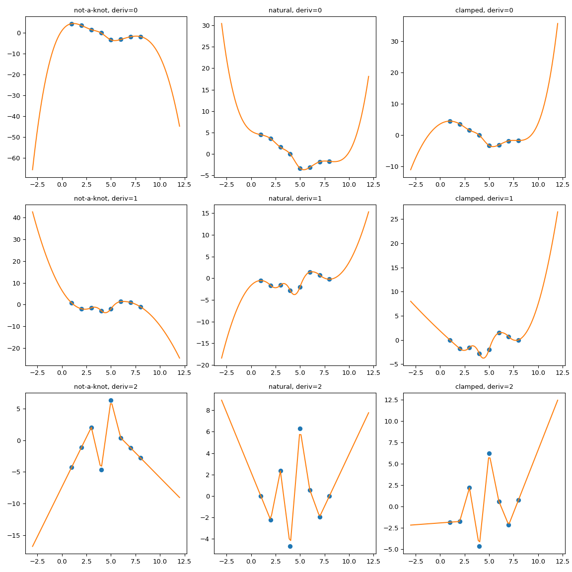
显然,自然样条在边界处确实具有零二阶导数,但外推是非线性的。bc_type="clamped" 也显示出类似的行为:一阶导数仅在边界处精确为零。在所有情况下,外推都是通过扩展样条的第一个和最后一个多项式段来完成的,无论它们是什么。
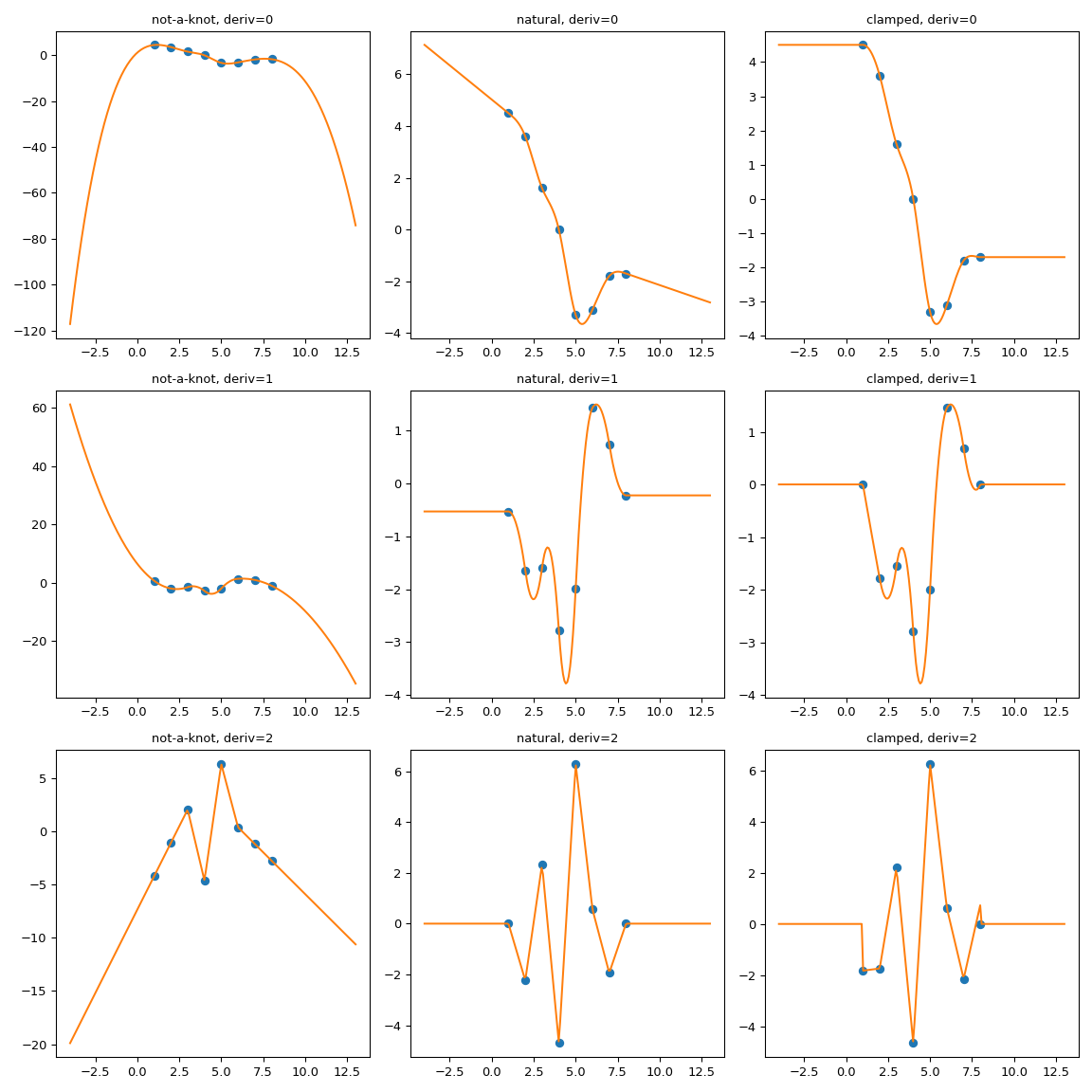
强制外推的一种可能方法是扩展插值域,以添加具有所需性质的第一个和最后一个多项式段。
这里我们使用 CubicSpline 超类 PPoly 的 extend 方法来添加两个额外的断点,并确保附加的多项式段保持导数的值。然后,外推将使用这两个附加区间进行。
import numpy as np
import matplotlib.pyplot as plt
from scipy.interpolate import CubicSpline

def add_boundary_knots(spline):
    """
    Add knots infinitesimally to the left and right.

    Additional intervals are added to have zero 2nd and 3rd derivatives,
    and to maintain the first derivative from whatever boundary condition
    was selected. The spline is modified in place.
    """
    # determine the slope at the left edge
    leftx = spline.x[0]
    lefty = spline(leftx)
    leftslope = spline(leftx, nu=1)

    # add a new breakpoint just to the left and use the
    # known slope to construct the PPoly coefficients.
    leftxnext = np.nextafter(leftx, leftx - 1)
    leftynext = lefty + leftslope*(leftxnext - leftx)
    leftcoeffs = np.array([0, 0, leftslope, leftynext])
    spline.extend(leftcoeffs[..., None], np.r_[leftxnext])

    # repeat with additional knots to the right
    rightx = spline.x[-1]
    righty = spline(rightx)
    rightslope = spline(rightx,nu=1)
    rightxnext = np.nextafter(rightx, rightx + 1)
    rightynext = righty + rightslope * (rightxnext - rightx)
    rightcoeffs = np.array([0, 0, rightslope, rightynext])
    spline.extend(rightcoeffs[..., None], np.r_[rightxnext])

xs = [1, 2, 3, 4, 5, 6, 7, 8]
ys = [4.5, 3.6, 1.6, 0.0, -3.3, -3.1, -1.8, -1.7]

notaknot = CubicSpline(xs,ys, bc_type='not-a-knot')
# not-a-knot does not require additional intervals

natural = CubicSpline(xs,ys, bc_type='natural')
# extend the natural natural spline with linear extrapolating knots
add_boundary_knots(natural)

clamped = CubicSpline(xs,ys, bc_type='clamped')
# extend the clamped spline with constant extrapolating knots
add_boundary_knots(clamped)

xnew = np.linspace(min(xs) - 5, max(xs) + 5, 201)

fig, axs = plt.subplots(3, 3,figsize=(12,12))

splines = [notaknot, natural, clamped]
titles = ['not-a-knot', 'natural', 'clamped']

for i in [0, 1, 2]:
    for j, spline, title in zip(range(3), splines, titles):
        axs[i, j].plot(xs, spline(xs, nu=i),'o')
        axs[i, j].plot(xnew, spline(xnew, nu=i),'-')
        axs[i, j].set_title(f'{title}, deriv={i}')

plt.tight_layout()
plt.show()
手动实现渐近线#
前面扩展插值域的技巧依赖于 CubicSpline.extend 方法。一个更为通用的替代方案是实现一个包装器,显式处理超出界限的行为。让我们考虑一个实际的例子。
设置#
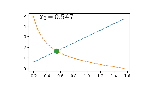
假设我们想在给定的 \(a\) 值下解方程
(这些方程的一种应用是求解量子粒子的能级)。为简单起见,我们只考虑 \(x\in (0, \pi/2)\)。
一次求解此方程很简单
import numpy as np
import matplotlib.pyplot as plt
from scipy.optimize import brentq

def f(x, a):
    return a*x - 1/np.tan(x)

a = 3
x0 = brentq(f, 1e-16, np.pi/2, args=(a,))   # here we shift the left edge
                                            # by a machine epsilon to avoid
                                            # a division by zero at x=0
xx = np.linspace(0.2, np.pi/2, 101)
plt.plot(xx, a*xx, '--')
plt.plot(xx, 1/np.tan(xx), '--')
plt.plot(x0, a*x0, 'o', ms=12)
plt.text(0.1, 0.9, fr'$x_0 = {x0:.3f}$',
               transform=plt.gca().transAxes, fontsize=16)
plt.show()
然而,如果我们需要多次求解(例如,由于 tan 函数的周期性而找到一系列根),重复调用 scipy.optimize.brentq 会变得非常昂贵。
为了规避这个困难,我们列出 \(y = ax - 1/\tan{x}\),并在列表网格上进行插值。实际上,我们将使用逆插值:我们插值 \(x\) 对 \(y\) 的值。这样,求解原始方程就变成了简单地评估插值函数在零 \(y\) 参数处的值。
为了提高插值精度,我们将利用列表函数导数的知识。我们将使用 BPoly.from_derivatives 来构造一个三次插值(等效地,我们可以使用 CubicHermiteSpline)。
import numpy as np
import matplotlib.pyplot as plt
from scipy.interpolate import BPoly

def f(x, a):
    return a*x - 1/np.tan(x)

xleft, xright = 0.2, np.pi/2
x = np.linspace(xleft, xright, 11)

fig, ax = plt.subplots(1, 2, figsize=(12, 4))

for j, a in enumerate([3, 93]):
    y = f(x, a)
    dydx = a + 1./np.sin(x)**2    # d(ax - 1/tan(x)) / dx
    dxdy = 1 / dydx               # dx/dy = 1 / (dy/dx)

    xdx = np.c_[x, dxdy]
    spl = BPoly.from_derivatives(y, xdx)   # inverse interpolation

    yy = np.linspace(f(xleft, a), f(xright, a), 51)
    ax[j].plot(yy, spl(yy), '--')
    ax[j].plot(y, x, 'o')
    ax[j].set_xlabel(r'$y$')
    ax[j].set_ylabel(r'$x$')
    ax[j].set_title(rf'$a = {a}$')

    ax[j].plot(0, spl(0), 'o', ms=12)
    ax[j].text(0.1, 0.85, fr'$x_0 = {spl(0):.3f}$',
               transform=ax[j].transAxes, fontsize=18)
    ax[j].grid(True)
plt.tight_layout()
plt.show()
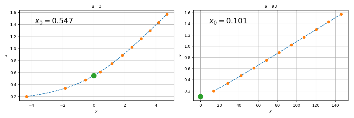
请注意,对于 \(a=3\),spl(0) 与上面的 brentq 调用一致,而对于 \(a = 93\),差异显著。该过程在 \(a\) 值过大时开始失效的原因是直线 \(y = ax\) 趋向于垂直轴,并且原始方程的根趋向于 \(x=0\)。由于我们在有限网格上列表了原始函数,spl(0) 涉及到对过大 \(a\) 值的推断。依赖推断容易丧失精度,最好避免。
利用已知渐近线#
查看原始方程,我们注意到当 \(x\to 0\) 时,\(\tan(x) = x + O(x^3)\),原始方程变为
因此对于 \(a \gg 1\),\(x_0 \approx 1/\sqrt{a}\)。
我们将利用这一点来创建一个类,该类将从插值切换到使用这种已知的渐近行为来处理超出范围的数据。一个最简单的实现可能如下所示
class RootWithAsymptotics:
   def __init__(self, a):

       # construct the interpolant
       xleft, xright = 0.2, np.pi/2
       x = np.linspace(xleft, xright, 11)

       y = f(x, a)
       dydx = a + 1./np.sin(x)**2    # d(ax - 1/tan(x)) / dx
       dxdy = 1 / dydx               # dx/dy = 1 / (dy/dx)

       # inverse interpolation
       self.spl = BPoly.from_derivatives(y, np.c_[x, dxdy])
       self.a = a

   def root(self):
       out = self.spl(0)
       asympt = 1./np.sqrt(self.a)
       return np.where(spl.x.min() < asympt, out, asympt)
然后
>>> r = RootWithAsymptotics(93)
>>> r.root()
array(0.10369517)
这与外推结果不同,但与 brentq 调用一致。
请注意,此实现是故意精简的。从 API 角度来看,您可能希望实现 __call__ 方法,以便 x 对 y 的完整依赖关系可用。从数值角度来看,需要更多工作来确保插值和渐近线之间的切换发生在渐近区域足够深处,以便结果函数在切换点处足够平滑。
此外,在此示例中,我们人为地将问题限制为仅考虑 tan 函数的单个周期区间,并且只处理 \(a > 0\)。对于 \(a\) 的负值,我们需要实现其他渐近线,例如 \(x\to \pi\)。
然而,基本思想是相同的。
D > 1 中的外推#
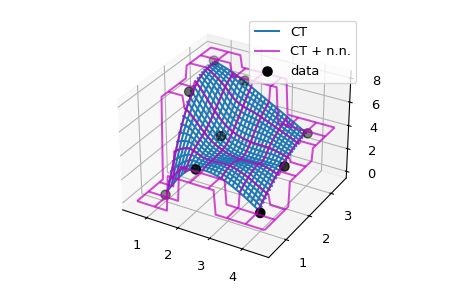
在包装器类或函数中手动实现外推的基本思想可以很容易地推广到更高维度。例如,我们考虑使用 CloughTocher2DInterpolator 对 2D 数据进行 C1 平滑插值。默认情况下,它将超出边界的值填充为 nan,而我们希望改为对每个查询点使用其最近邻居的值。
由于 CloughTocher2DInterpolator 接受 2D 数据或数据点的 Delaunay 三角剖分,因此查找查询点最近邻的有效方法是构建三角剖分(使用 scipy.spatial 工具)并使用它在数据的凸包上查找最近邻。
我们将改用更简单、更直接的方法,并依赖于使用 NumPy 广播遍历整个数据集。
import numpy as np
import matplotlib.pyplot as plt
from scipy.interpolate import CloughTocher2DInterpolator as CT

def my_CT(xy, z):
    """CT interpolator + nearest-neighbor extrapolation.

    Parameters
    ----------
    xy : ndarray, shape (npoints, ndim)
        Coordinates of data points
    z : ndarray, shape (npoints)
        Values at data points

    Returns
    -------
    func : callable
        A callable object which mirrors the CT behavior,
        with an additional neareast-neighbor extrapolation
        outside of the data range.
    """
    x = xy[:, 0]
    y = xy[:, 1]
    f = CT(xy, z)

    # this inner function will be returned to a user
    def new_f(xx, yy):
        # evaluate the CT interpolator. Out-of-bounds values are nan.
        zz = f(xx, yy)
        nans = np.isnan(zz)

        if nans.any():
            # for each nan point, find its nearest neighbor
            inds = np.argmin(
                (x[:, None] - xx[nans])**2 +
                (y[:, None] - yy[nans])**2
                , axis=0)
            # ... and use its value
            zz[nans] = z[inds]
        return zz

    return new_f

# Now illustrate the difference between the original ``CT`` interpolant
# and ``my_CT`` on a small example:

x = np.array([1, 1, 1, 2, 2, 2, 4, 4, 4])
y = np.array([1, 2, 3, 1, 2, 3, 1, 2, 3])
z = np.array([0, 7, 8, 3, 4, 7, 1, 3, 4])

xy = np.c_[x, y]
lut = CT(xy, z)
lut2 = my_CT(xy, z)

X = np.linspace(min(x) - 0.5, max(x) + 0.5, 71)
Y = np.linspace(min(y) - 0.5, max(y) + 0.5, 71)
X, Y = np.meshgrid(X, Y)

fig = plt.figure()
ax = fig.add_subplot(projection='3d')

ax.plot_wireframe(X, Y, lut(X, Y), label='CT')
ax.plot_wireframe(X, Y, lut2(X, Y), color='m',
                  cstride=10, rstride=10, alpha=0.7, label='CT + n.n.')

ax.scatter(x, y, z,  'o', color='k', s=48, label='data')
ax.legend()
plt.tight_layout()