interp2d 转换指南

本页包含三组示例

• 用于 scipy.interpolate.interp2d 的底层 FITPACK 替代品，用于与旧版 scipy.interpolate.interp2d 错误兼容的替代品；

• 在新代码中推荐用于 scipy.interpolate.interp2d 的替代品；

• 二维基于 FITPACK 的线性插值的失败模式演示以及推荐的替代品。

1. 如何逐步停止使用 interp2d

interp2d 会在二维规则网格上的插值和二维散点数据插值之间静默切换。这种切换是基于 (展平的) x、y 和 z 数组的长度。简而言之，对于规则网格，请使用 scipy.interpolate.RectBivariateSpline；对于散点插值，请使用 bisprep/bisplev 组合。下面我们将给出逐点转换的示例，这应该能精确地保留 interp2d 的结果。

1.1 在规则网格上使用 interp2d

我们从（略微修改的）文档字符串示例开始。

>>> import numpy as np
>>> import matplotlib.pyplot as plt
>>> from scipy.interpolate import interp2d, RectBivariateSpline

>>> x = np.arange(-5.01, 5.01, 0.25)
>>> y = np.arange(-5.01, 7.51, 0.25)
>>> xx, yy = np.meshgrid(x, y)
>>> z = np.sin(xx**2 + 2.*yy**2)
>>> f = interp2d(x, y, z, kind='cubic')

这是“规则网格”代码路径，因为

>>> z.size == len(x) * len(y)
True

另外，请注意 x.size != y.size

>>> x.size, y.size
(41, 51)

现在，我们构建一个便利函数来构造插值器并绘制它。

>>> def plot(f, xnew, ynew):
...    fig, (ax1, ax2) = plt.subplots(1, 2, figsize=(8, 4))
...    znew = f(xnew, ynew)
...    ax1.plot(x, z[0, :], 'ro-', xnew, znew[0, :], 'b-')
...    im = ax2.imshow(znew)
...    plt.colorbar(im, ax=ax2)
...    plt.show()
...    return znew
...
>>> xnew = np.arange(-5.01, 5.01, 1e-2)
>>> ynew = np.arange(-5.01, 7.51, 1e-2)
>>> znew_i = plot(f, xnew, ynew)

替代方案：使用 RectBivariateSpline，结果是相同的

请注意转置：首先，在构造函数中；其次，您需要转置评估结果。这是为了撤消 interp2d 所做的转置。

>>> r = RectBivariateSpline(x, y, z.T)
>>> rt = lambda xnew, ynew: r(xnew, ynew).T
>>> znew_r = plot(rt, xnew, ynew)

>>> from numpy.testing import assert_allclose
>>> assert_allclose(znew_i, znew_r, atol=1e-14)

插值阶数：线性、三次等

interp2d 默认为 kind="linear"，即在 x- 和 y- 两个方向上都是线性的。另一方面，RectBivariateSpline 默认为三次插值，即 kx=3, ky=3。

以下是精确的等价关系

interp2d	RectBivariateSpline
无 kwargs	kx = 1, ky = 1
kind=’linear’	kx = 1, ky = 1
kind=’cubic’	kx = 3, ky = 3

1.2. 具有完整点坐标的 interp2d（散点插值）

这里，我们展平了上一个练习中的网格，以说明其功能。

>>> xxr = xx.ravel()
>>> yyr = yy.ravel()
>>> zzr = z.ravel()
>>> f = interp2d(xxr, yyr, zzr, kind='cubic')

请注意，这是“非规则网格”代码路径，适用于散点数据，其中 len(x) == len(y) == len(z)。

>>> len(xxr) == len(yyr) == len(zzr)
True

>>> xnew = np.arange(-5.01, 5.01, 1e-2)
>>> ynew = np.arange(-5.01, 7.51, 1e-2)
>>> znew_i = plot(f, xnew, ynew)

替代方案：直接使用 scipy.interpolate.bisplrep / scipy.interpolate.bisplev

>>> from scipy.interpolate import bisplrep, bisplev
>>> tck = bisplrep(xxr, yyr, zzr, kx=3, ky=3, s=0)
# convenience: make up a callable from bisplev
>>> ff = lambda xnew, ynew: bisplev(xnew, ynew, tck).T   # Note the transpose, to mimic what interp2d does
>>> znew_b = plot(ff, xnew, ynew)

>>> assert_allclose(znew_i, znew_b, atol=1e-15)

插值阶数：线性、三次等

interp2d 默认为 kind="linear"，即在 x- 和 y- 两个方向上都是线性的。另一方面，bisplrep 默认为三次插值，即 kx=3, ky=3。

以下是精确的等价关系

interp2d	bisplrep
无 kwargs	kx = 1, ky = 1
kind=’linear’	kx = 1, ky = 1
kind=’cubic’	kx = 3, ky = 3

2. interp2d 的替代方案：规则网格

对于新代码，推荐的替代方案是 RegularGridInterpolator。它是一个独立的实现，不基于 FITPACK。支持最近邻、线性插值和奇数阶张量积样条。

样条结节保证与数据点重合。

请注意，这里

1. 元组参数是 (x, y)

2. z 数组需要转置

3. 关键字名称是 method，而不是 kind

4. bounds_error 参数默认为 True。

>>> from scipy.interpolate import RegularGridInterpolator as RGI
>>> r = RGI((x, y), z.T, method='linear', bounds_error=False)

评估：创建一个二维网格。使用 `indexing='ij'` 和 sparse=True 来节省内存

>>> xxnew, yynew = np.meshgrid(xnew, ynew, indexing='ij', sparse=True)

评估时，请注意元组参数

>>> znew_reggrid = r((xxnew, yynew))

>>> fig, (ax1, ax2) = plt.subplots(1, 2, figsize=(8, 4))
# Again, note the transpose to undo the `interp2d` convention
>>> znew_reggrid_t = znew_reggrid.T
>>> ax1.plot(x, z[0, :], 'ro-', xnew, znew_reggrid_t[0, :], 'b-')
>>> im = ax2.imshow(znew_reggrid_t)
>>> plt.colorbar(im, ax=ax2)

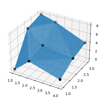
3. 散点二维线性插值：优先使用 LinearNDInterpolator 而非 SmoothBivariateSpline 或 bisplrep

对于二维散点线性插值，SmoothBivariateSpline 和 bisplrep 都可能发出警告、未能插值数据，或者生成结节偏离数据点的样条。因此，推荐使用基于 QHull 对数据进行三角剖分的 LinearNDInterpolator。

# TestSmoothBivariateSpline::test_integral
>>> from scipy.interpolate import SmoothBivariateSpline, LinearNDInterpolator
>>> x = np.array([1,1,1,2,2,2,4,4,4])
>>> y = np.array([1,2,3,1,2,3,1,2,3])
>>> z = np.array([0,7,8,3,4,7,1,3,4])

现在，使用基于 Qhull 的数据三角剖分进行线性插值

>>> xy = np.c_[x, y]   # or just list(zip(x, y))
>>> lut2 = LinearNDInterpolator(xy, z)
>>> X = np.linspace(min(x), max(x))
>>> Y = np.linspace(min(y), max(y))
>>> X, Y = np.meshgrid(X, Y)

结果易于理解和解释

>>> fig = plt.figure()
>>> ax = fig.add_subplot(projection='3d')
>>> ax.plot_wireframe(X, Y, lut2(X, Y))
>>> ax.scatter(x, y, z,  'o', color='k', s=48)

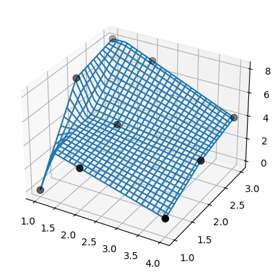
请注意，bisplrep 的行为有所不同！它可能会将样条结节放置在数据范围之外。

为了说明，考虑与上一个示例相同的数据

>>> tck = bisplrep(x, y, z, kx=1, ky=1, s=0)
>>> fig = plt.figure()
>>> ax = fig.add_subplot(projection='3d')
>>> xx = np.linspace(min(x), max(x))
>>> yy = np.linspace(min(y), max(y))
>>> X, Y = np.meshgrid(xx, yy)
>>> Z = bisplev(xx, yy, tck)
>>> Z = Z.reshape(*X.shape).T
>>> ax.plot_wireframe(X, Y, Z, rstride=2, cstride=2)
>>> ax.scatter(x, y, z,  'o', color='k', s=48)

此外，SmoothBivariateSpline 未能插值数据。同样，使用与上一个示例相同的数据。

>>> lut = SmoothBivariateSpline(x, y, z, kx=1, ky=1, s=0)
>>> fig = plt.figure()
>>> ax = fig.add_subplot(projection='3d')
>>> xx = np.linspace(min(x), max(x))
>>> yy = np.linspace(min(y), max(y))
>>> X, Y = np.meshgrid(xx, yy)
>>> ax.plot_wireframe(X, Y, lut(xx, yy).T, rstride=4, cstride=4)
>>> ax.scatter(x, y, z,  'o', color='k', s=48)

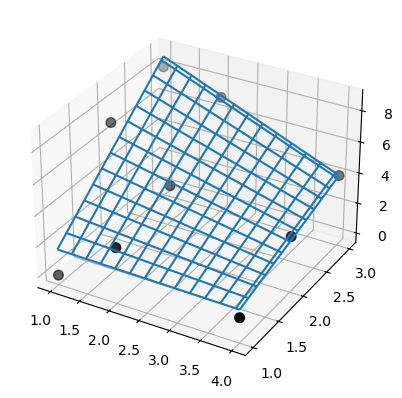
请注意，SmoothBivariateSpline 和 bisplrep 的结果都存在伪影，这与 LinearNDInterpolator 的结果不同。此处所示问题曾被报告存在于线性插值中，但 FITPACK 结节选择机制并不能保证在高阶（例如三次）样条曲面中避免这些问题。