scipy.special.stdtr#

scipy.special.stdtr(df, t, out=None) = <ufunc 'stdtr'>#

学生 t 分布累积分布函数

返回积分

\[\frac{\Gamma((df+1)/2)}{\sqrt{\pi df} \Gamma(df/2)} \int_{-\infty}^t (1+x^2/df)^{-(df+1)/2}\, dx\]

参数:

dfarray_like: 自由度
tarray_like: 积分上限
outndarray, optional: 函数结果的可选输出数组

返回:

标量或 ndarray: 在 t 处的学生 t CDF 值

另请参见

stdtridf: stdtr 关于 df 的逆函数
stdtrit: stdtr 关于 t 的逆函数
scipy.stats.t: 学生 t 分布

说明

学生 t 分布也可通过 scipy.stats.t 获得。直接调用 stdtr 可以比调用 scipy.stats.t 的 cdf 方法提高性能（参见下面的最后一个示例）。

除了 NumPy 之外，stdtr 对 Python 数组 API 标准兼容的后端提供实验性支持。请考虑通过设置环境变量 SCIPY_ARRAY_API=1 并提供 CuPy、PyTorch、JAX 或 Dask 数组作为数组参数来测试这些功能。支持以下后端和设备（或其他功能）的组合。

库	CPU	GPU
NumPy	✅	不适用
CuPy	不适用	✅
PyTorch	✅	⛔
JAX	✅	✅
Dask	✅	不适用

有关更多信息，请参阅对数组 API 标准的支持。

示例

计算 df=3 在 t=1 处的函数。

>>> import numpy as np
>>> from scipy.special import stdtr
>>> import matplotlib.pyplot as plt
>>> stdtr(3, 1)
0.8044988905221148

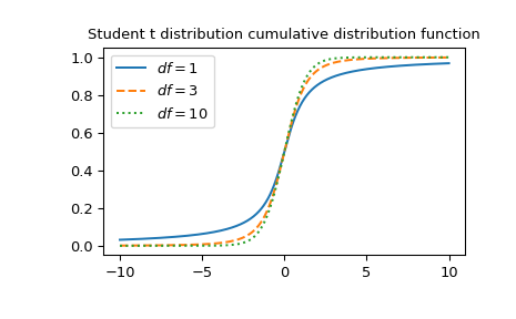
绘制三种不同自由度下的函数。

>>> x = np.linspace(-10, 10, 1000)
>>> fig, ax = plt.subplots()
>>> parameters = [(1, "solid"), (3, "dashed"), (10, "dotted")]
>>> for (df, linestyle) in parameters:
...     ax.plot(x, stdtr(df, x), ls=linestyle, label=f"$df={df}$")
>>> ax.legend()
>>> ax.set_title("Student t distribution cumulative distribution function")
>>> plt.show()

../../_images/scipy-special-stdtr-1_00_00.png

通过为 df 提供 NumPy 数组或列表，可以同时计算多个自由度下的函数。

>>> stdtr([1, 2, 3], 1)
array([0.75      , 0.78867513, 0.80449889])

通过为 df 和 t 提供形状兼容以进行广播的数组，可以同时计算多个不同自由度下多个点的函数。计算 3 个自由度在 4 个点处的 stdtr，得到一个形状为 3x4 的数组。

>>> dfs = np.array([[1], [2], [3]])
>>> t = np.array([2, 4, 6, 8])
>>> dfs.shape, t.shape
((3, 1), (4,))

>>> stdtr(dfs, t)
array([[0.85241638, 0.92202087, 0.94743154, 0.96041658],
       [0.90824829, 0.97140452, 0.98666426, 0.99236596],
       [0.93033702, 0.98599577, 0.99536364, 0.99796171]])

t 分布也可通过 scipy.stats.t 获得。直接调用 stdtr 可能比调用 scipy.stats.t 的 cdf 方法快得多。为了获得相同的结果，必须使用以下参数化：scipy.stats.t(df).cdf(x) = stdtr(df, x)。

>>> from scipy.stats import t
>>> df, x = 3, 1
>>> stdtr_result = stdtr(df, x)  # this can be faster than below
>>> stats_result = t(df).cdf(x)
>>> stats_result == stdtr_result  # test that results are equal
True