scipy.special.fdtrc#

scipy.special.fdtrc(dfn, dfd, x, out=None) = <ufunc 'fdtrc'>#

F 生存函数。

返回互补 F 分布函数（密度从 x 到无穷大的积分）。

参数:

dfnarray_like: 第一个参数（正浮点数）。
dfdarray_like: 第二个参数（正浮点数）。
xarray_like: 参数（非负浮点数）。
outndarray, optional: 函数值的可选输出数组

返回:

y标量或 ndarray: 具有参数 dfn 和 dfd 在 x 处的互补 F 分布函数。

参见

fdtr: F 分布累积分布函数
fdtri: F 分布逆累积分布函数
scipy.stats.f: F 分布

注释

使用正则化不完全 Beta 函数，根据公式：

\[F(d_n, d_d; x) = I_{d_d/(d_d + xd_n)}(d_d/2, d_n/2).\]

Cephes [1] 例程 fdtrc 的包装器。 F 分布也可作为 scipy.stats.f 使用。与 scipy.stats.f 的 sf 方法相比，直接调用 fdtrc 可以提高性能（参见下面的最后一个示例）。

参考文献

[1]

Cephes 数学函数库，http://www.netlib.org/cephes/

示例

计算 dfn=1 和 dfd=2 在 x=1 处的函数值。

>>> import numpy as np
>>> from scipy.special import fdtrc
>>> fdtrc(1, 2, 1)
0.42264973081037427

通过为 x 提供 NumPy 数组来计算多个点的函数值。

>>> x = np.array([0.5, 2., 3.])
>>> fdtrc(1, 2, x)
array([0.5527864 , 0.29289322, 0.22540333])

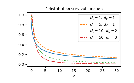
绘制多个参数集的函数图。

>>> import matplotlib.pyplot as plt
>>> dfn_parameters = [1, 5, 10, 50]
>>> dfd_parameters = [1, 1, 2, 3]
>>> linestyles = ['solid', 'dashed', 'dotted', 'dashdot']
>>> parameters_list = list(zip(dfn_parameters, dfd_parameters,
...                            linestyles))
>>> x = np.linspace(0, 30, 1000)
>>> fig, ax = plt.subplots()
>>> for parameter_set in parameters_list:
...     dfn, dfd, style = parameter_set
...     fdtrc_vals = fdtrc(dfn, dfd, x)
...     ax.plot(x, fdtrc_vals, label=rf"$d_n={dfn},\, d_d={dfd}$",
...             ls=style)
>>> ax.legend()
>>> ax.set_xlabel("$x$")
>>> ax.set_title("F distribution survival function")
>>> plt.show()

../../_images/scipy-special-fdtrc-1_00_00.png

F 分布也可作为 scipy.stats.f 使用。直接使用 fdtrc 比调用 scipy.stats.f 的 sf 方法快得多，特别是对于小型数组或单个值。要获得相同的结果，必须使用以下参数化： stats.f(dfn, dfd).sf(x)=fdtrc(dfn, dfd, x)。

>>> from scipy.stats import f
>>> dfn, dfd = 1, 2
>>> x = 1
>>> fdtrc_res = fdtrc(dfn, dfd, x)  # this will often be faster than below
>>> f_dist_res = f(dfn, dfd).sf(x)
>>> f_dist_res == fdtrc_res  # test that results are equal
True