scipy.signal.

correlate#

scipy.signal.correlate(in1, in2, mode='full', method='auto')[source]#

对两个 N 维数组进行互相关。

对 in1 和 in2 进行互相关，输出大小由 mode 参数决定。

参数:

in1array_like

第一个输入。

in2array_like

第二个输入。应与 in1 具有相同的维度数。

modestr {‘full’, ‘valid’, ‘same’}, 可选

一个字符串，指示输出的大小

full: 输出是输入的完整离散线性互相关。(默认)
valid: 输出仅包含那些不依赖零填充的元素。在 'valid' 模式下，in1 或 in2 必须在每个维度上至少与另一个一样大。
same: 输出大小与 in1 相同，并相对于 'full' 输出居中。

methodstr {‘auto’, ‘direct’, ‘fft’}, 可选

一个字符串，指示用于计算相关性的方法。

direct: 相关性直接根据求和（相关性的定义）确定。
fft: 快速傅里叶变换用于更快地执行相关性计算（仅适用于数值数组）。
auto: 根据对速度的估计，自动选择直接法或傅里叶法（默认）。有关更多详细信息，请参阅 convolve 注释。

0.19.0 版本新增。

返回:

correlatearray: 一个 N 维数组，包含 in1 与 in2 的离散线性互相关的一个子集。

另请参阅

choose_conv_method: 包含有关 method 的更多文档。
correlation_lags: 计算一维互相关的时间滞后/位移索引数组。

备注

两个 d 维数组 x 和 y 的相关性 z 定义为

z[...,k,...] = sum[..., i_l, ...] x[..., i_l,...] * conj(y[..., i_l - k,...])

这样，如果 x 和 y 是一维数组，并且 z = correlate(x, y, 'full')，则

\[z[k] = \sum_{l=0}^{N-1} x_l \, y_{l-k}^{*}\]

对于 \(k = -(M-1), \dots, (N-1)\)，其中 \(N\) 是 x 的长度，\(M\) 是 y\) 的长度，当 \(m\) 超出有效范围 \([0, M-1]\) 时 \(y_m = 0\)。\(z\) 的大小是 \(N + M - 1\)，\(y^*\) 表示 \(y\) 的复共轭。


method='fft' 仅适用于数值数组，因为它依赖于 fftconvolve。在某些情况下（即，对象数组或整数取整可能导致精度损失时），始终使用 method='direct'。
当对偶数长度输入使用 mode='same' 时，correlate 和 correlate2d 的输出会有所不同：它们之间存在一个索引偏移。
示例


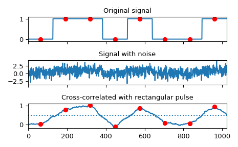
使用互相关实现匹配滤波器，以恢复通过噪声通道的信号。
>>> import numpy as np
>>> from scipy import signal
>>> import matplotlib.pyplot as plt
>>> rng = np.random.default_rng()


>>> sig = np.repeat([0., 1., 1., 0., 1., 0., 0., 1.], 128)
>>> sig_noise = sig + rng.standard_normal(len(sig))
>>> corr = signal.correlate(sig_noise, np.ones(128), mode='same') / 128


>>> clock = np.arange(64, len(sig), 128)
>>> fig, (ax_orig, ax_noise, ax_corr) = plt.subplots(3, 1, sharex=True)
>>> ax_orig.plot(sig)
>>> ax_orig.plot(clock, sig[clock], 'ro')
>>> ax_orig.set_title('Original signal')
>>> ax_noise.plot(sig_noise)
>>> ax_noise.set_title('Signal with noise')
>>> ax_corr.plot(corr)
>>> ax_corr.plot(clock, corr[clock], 'ro')
>>> ax_corr.axhline(0.5, ls=':')
>>> ax_corr.set_title('Cross-correlated with rectangular pulse')
>>> ax_orig.margins(0, 0.1)
>>> fig.tight_layout()
>>> plt.show()





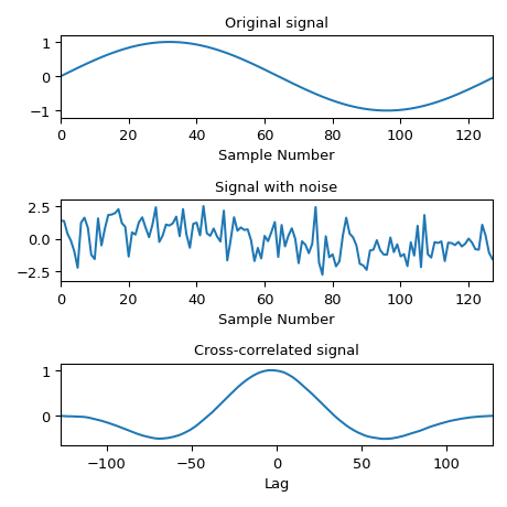
计算噪声信号与原始信号的互相关。
>>> x = np.arange(128) / 128
>>> sig = np.sin(2 * np.pi * x)
>>> sig_noise = sig + rng.standard_normal(len(sig))
>>> corr = signal.correlate(sig_noise, sig)
>>> lags = signal.correlation_lags(len(sig), len(sig_noise))
>>> corr /= np.max(corr)


>>> fig, (ax_orig, ax_noise, ax_corr) = plt.subplots(3, 1, figsize=(4.8, 4.8))
>>> ax_orig.plot(sig)
>>> ax_orig.set_title('Original signal')
>>> ax_orig.set_xlabel('Sample Number')
>>> ax_noise.plot(sig_noise)
>>> ax_noise.set_title('Signal with noise')
>>> ax_noise.set_xlabel('Sample Number')
>>> ax_corr.plot(lags, corr)
>>> ax_corr.set_title('Cross-correlated signal')
>>> ax_corr.set_xlabel('Lag')
>>> ax_orig.margins(0, 0.1)
>>> ax_noise.margins(0, 0.1)
>>> ax_corr.margins(0, 0.1)
>>> fig.tight_layout()
>>> plt.show()


              
              
              
              
              
                
                  

       上一页
 convolve
 
    下一页
 fftconvolve