scipy.signal.

correlate2d

scipy.signal.correlate2d(in1, in2, mode='full', boundary='fill', fillvalue=0)

对两个二维数组进行互相关运算。

使用由 mode 确定的输出大小，以及由 boundary 和 fillvalue 确定的边界条件，对 in1 和 in2 进行互相关运算。

参数:

in1类数组

第一个输入。

in2类数组

第二个输入。应与 in1 具有相同的维度数。

mode字符串 {‘full’, ‘valid’, ‘same’}, 可选

一个字符串，指示输出的大小

full

输出为输入的完整离散线性互相关结果。(默认)

valid

输出仅包含不依赖于零填充的元素。在“valid”模式下，in1 或 in2 必须在每个维度上至少与另一个一样大。

same

输出大小与 in1 相同，并相对于“full”输出居中。

boundary字符串 {‘fill’, ‘wrap’, ‘symm’}, 可选

一个标志，指示如何处理边界

fill

用 fillvalue 填充输入数组。(默认)

wrap

循环边界条件。

symm

对称边界条件。

fillvalue标量, 可选

用于填充输入数组的值。默认为 0。

返回:

correlate2dndarray

一个二维数组，包含 in1 和 in2 的离散线性互相关结果的子集。

注意

当对偶数长度的输入使用“same”模式时，correlate 和 correlate2d 的输出会有所不同：它们之间存在一个1索引的偏移。

示例

在浏览器中尝试！

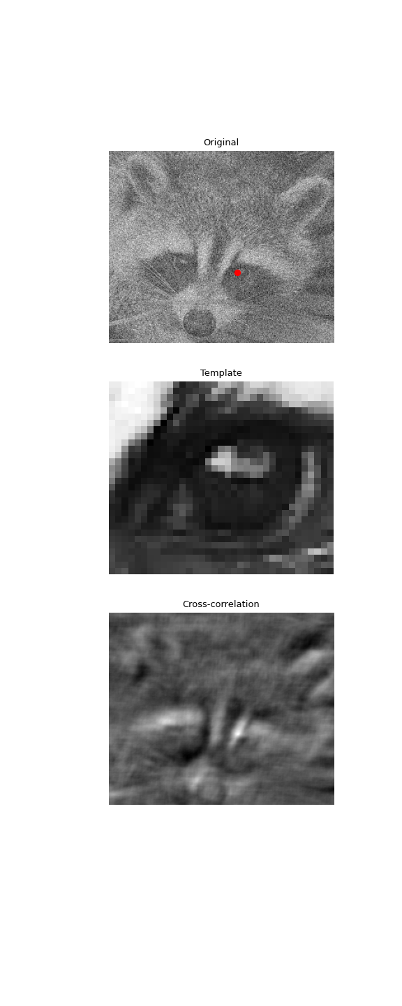
使用二维互相关在噪声图像中查找模板位置

>>> import numpy as np
>>> from scipy import signal, datasets, ndimage
>>> rng = np.random.default_rng()
>>> face = datasets.face(gray=True) - datasets.face(gray=True).mean()
>>> face = ndimage.zoom(face[30:500, 400:950], 0.5)  # extract the face
>>> template = np.copy(face[135:165, 140:175])  # right eye
>>> template -= template.mean()
>>> face = face + rng.standard_normal(face.shape) * 50  # add noise
>>> corr = signal.correlate2d(face, template, boundary='symm', mode='same')
>>> y, x = np.unravel_index(np.argmax(corr), corr.shape)  # find the match

>>> import matplotlib.pyplot as plt
>>> fig, (ax_orig, ax_template, ax_corr) = plt.subplots(3, 1,
...                                                     figsize=(6, 15))
>>> ax_orig.imshow(face, cmap='gray')
>>> ax_orig.set_title('Original')
>>> ax_orig.set_axis_off()
>>> ax_template.imshow(template, cmap='gray')
>>> ax_template.set_title('Template')
>>> ax_template.set_axis_off()
>>> ax_corr.imshow(corr, cmap='gray')
>>> ax_corr.set_title('Cross-correlation')
>>> ax_corr.set_axis_off()
>>> ax_orig.plot(x, y, 'ro')
>>> fig.show()

返回在新标签页中打开