bootstrap#
- scipy.stats.bootstrap(data, statistic, *, n_resamples=9999, batch=None, vectorized=None, paired=False, axis=0, confidence_level=0.95, alternative='two-sided', method='BCa', bootstrap_result=None, rng=None)[source]#
计算统计量的双边 bootstrap 置信区间。
当 method 为
'percentile'且 alternative 为'two-sided'时,bootstrap 置信区间按照以下步骤计算。重采样数据:对于 data 中的每个样本,以及对于每个 n_resamples,从原始样本中抽取与原始样本大小相同的随机样本(带放回)。
计算统计量的 bootstrap 分布:对于每组重采样,计算检验统计量。
确定置信区间:找到 bootstrap 分布的区间,该区间
关于中位数对称,并且
包含 confidence_level 的重采样统计量值。
虽然
'percentile'方法是最直观的,但它在实践中很少使用。还有两种更常用的方法可用,'basic'(“反向百分位数”)和'BCa'(“偏差校正和加速”);它们在执行步骤 3 的方式上有所不同。如果 data 中的样本是从它们各自的分布中随机抽取的 \(n\) 次,则
bootstrap返回的置信区间将包含这些分布的统计量的真实值大约 confidence_level\(\, \times \, n\) 次。- 参数:
- data类数组序列
data 的每个元素都是一个样本,包含来自底层分布的标量观测值。 data 的元素必须可广播到相同的形状(可能除了由 axis 指定的维度)。
- statistic可调用对象
要计算置信区间的统计量。 statistic 必须是一个可调用对象,它接受
len(data)个样本作为单独的参数,并返回结果统计量。 如果 vectorized 设置为True,则 statistic 还必须接受一个关键字参数 axis,并且进行向量化以计算沿提供的 axis 的统计量。- n_resamplesint,默认值:
9999 执行的重采样次数,以形成统计量的 bootstrap 分布。
- batchint,可选
每次对 statistic 进行向量化调用时要处理的重采样数。 内存使用量为 O( batch *
n),其中n是样本大小。 默认值为None,在这种情况下,batch = n_resamples(对于method='BCa',则batch = max(n_resamples, n))。- vectorizedbool,可选
如果 vectorized 设置为
False,则不会将关键字参数 axis 传递给 statistic,并且期望仅为 1D 样本计算统计量。 如果True,则将关键字参数 axis 传递给 statistic,并且期望在传递 ND 样本数组时沿 axis 计算统计量。 如果None(默认),如果axis是 statistic 的参数,则将 vectorized 设置为True。 使用向量化统计量通常会减少计算时间。- pairedbool,默认值:
False 统计量是否将 data 中样本的对应元素视为配对的。 如果为 True,
bootstrap重采样 indices 的数组,并对 data 中的所有数组使用相同的索引; 否则,bootstrap独立地重采样每个数组的元素。- axisint,默认值:
0 样本在 data 中的轴,沿该轴计算 statistic。
- confidence_levelfloat,默认值:
0.95 置信区间的置信水平。
- alternative{‘two-sided’,‘less’,‘greater’},默认值:
'two-sided' 选择
'two-sided'(默认)用于双边置信区间,'less'用于下界为-np.inf的单边置信区间,以及'greater'用于上界为np.inf的单边置信区间。 单边置信区间的另一个界与双边置信区间的界相同,confidence_level 与 1.0 的距离是两倍; 例如,95%'less'置信区间的上界与 90%'two-sided'置信区间的上界相同。- method{‘percentile’,‘basic’,‘bca’},默认值:
'BCa' 是返回“百分位数”bootstrap 置信区间 (
'percentile'),还是“基本”(又名“反向”)bootstrap 置信区间 ('basic'),还是偏差校正和加速的 bootstrap 置信区间 ('BCa')。- bootstrap_resultBootstrapResult,可选
提供先前调用
bootstrap返回的结果对象,以将先前的 bootstrap 分布包含在新的 bootstrap 分布中。 例如,这可用于更改 confidence_level,更改 method,或者查看执行额外重采样而不重复计算的效果。- rng{None,int,
numpy.random.Generator},可选 如果通过关键字传递 rng,则将
numpy.random.Generator以外的类型传递给numpy.random.default_rng以实例化Generator。 如果 rng 已经是Generator实例,则使用提供的实例。 指定 rng 以实现可重复的函数行为。如果此参数通过位置传递或 random_state 通过关键字传递,则应用参数 random_state 的旧行为
如果 random_state 为 None(或
numpy.random),则使用numpy.random.RandomState单例。如果 random_state 是 int,则使用一个新的
RandomState实例,并使用 random_state 作为种子。如果 random_state 已经是
Generator或RandomState实例,则使用该实例。
在版本 1.15.0 中更改:作为从使用
numpy.random.RandomState过渡到numpy.random.Generator的 SPEC-0007 过渡的一部分,此关键字从 random_state 更改为 rng。 在过渡期间,这两个关键字将继续有效,但一次只能指定一个。 在过渡期之后,使用 random_state 关键字的函数调用将发出警告。 上面概述了 random_state 和 rng 的行为,但在新代码中应仅使用 rng 关键字。
- 返回值:
- resBootstrapResult
具有属性的对象
- confidence_intervalConfidenceInterval
bootstrap 置信区间,作为具有属性 low 和 high 的
collections.namedtuple的实例。- bootstrap_distributionndarray
bootstrap 分布,即每个重采样的 statistic 值。 最后一个维度与重采样对应(例如,
res.bootstrap_distribution.shape[-1] == n_resamples)。- standard_errorfloat 或 ndarray
bootstrap 标准误差,即 bootstrap 分布的样本标准差。
- 警告:
DegenerateDataWarning当
method='BCa'并且 bootstrap 分布退化时(例如,所有元素都相同)生成。
注释
如果 bootstrap 分布退化(例如,所有元素都相同),则
method='BCa'的置信区间的元素可能为 NaN。 在这种情况下,请考虑使用另一种 method 或检查 data,以获取其他分析可能更合适的指示(例如,所有观测值都相同)。参考文献
[1]B. Efron 和 R. J. Tibshirani,《Bootstrap 简介》,Chapman & Hall/CRC,Boca Raton,FL,USA (1993)
[2]Nathaniel E. Helwig,“Bootstrap 置信区间”,http://users.stat.umn.edu/~helwig/notes/bootci-Notes.pdf
[3]自举(统计),维基百科,https://en.wikipedia.org/wiki/Bootstrapping_%28statistics%29
示例
假设我们已经从未知分布中采样了数据。
>>> import numpy as np
>>> rng = np.random.default_rng()
>>> from scipy.stats import norm
>>> dist = norm(loc=2, scale=4)  # our "unknown" distribution
>>> data = dist.rvs(size=100, random_state=rng)
我们对分布的标准差感兴趣。
>>> std_true = dist.std()      # the true value of the statistic
>>> print(std_true)
4.0
>>> std_sample = np.std(data)  # the sample statistic
>>> print(std_sample)
3.9460644295563863
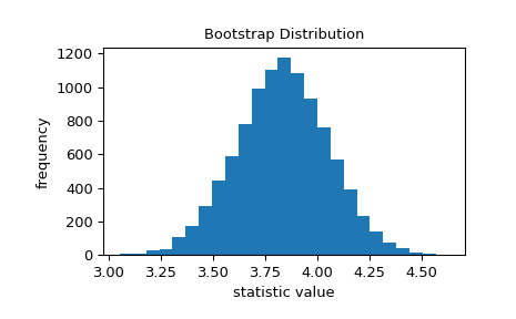
bootstrap 用于近似当我们重复从未知分布中采样并每次计算样本的统计量时,我们期望的可变性。 它通过重复地从原始样本中重采样值带放回,并计算每个重采样的统计量来实现这一点。 这导致统计量的“bootstrap 分布”。
>>> import matplotlib.pyplot as plt
>>> from scipy.stats import bootstrap
>>> data = (data,)  # samples must be in a sequence
>>> res = bootstrap(data, np.std, confidence_level=0.9, rng=rng)
>>> fig, ax = plt.subplots()
>>> ax.hist(res.bootstrap_distribution, bins=25)
>>> ax.set_title('Bootstrap Distribution')
>>> ax.set_xlabel('statistic value')
>>> ax.set_ylabel('frequency')
>>> plt.show()
标准误差量化了这种可变性。 它计算为 bootstrap 分布的标准差。
>>> res.standard_error
0.24427002125829136
>>> res.standard_error == np.std(res.bootstrap_distribution, ddof=1)
True
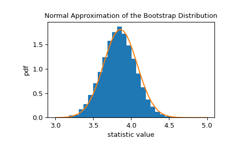
统计量的 bootstrap 分布通常近似于正态分布,其尺度等于标准误差。
>>> x = np.linspace(3, 5)
>>> pdf = norm.pdf(x, loc=std_sample, scale=res.standard_error)
>>> fig, ax = plt.subplots()
>>> ax.hist(res.bootstrap_distribution, bins=25, density=True)
>>> ax.plot(x, pdf)
>>> ax.set_title('Normal Approximation of the Bootstrap Distribution')
>>> ax.set_xlabel('statistic value')
>>> ax.set_ylabel('pdf')
>>> plt.show()
这表明我们可以基于此正态分布的分位数构造统计量的 90% 置信区间。
>>> norm.interval(0.9, loc=std_sample, scale=res.standard_error)
(3.5442759991341726, 4.3478528599786)
由于中心极限定理,此正态近似对于样本基础的各种统计量和分布是准确的; 但是,该近似在所有情况下都不可靠。 因为
bootstrap旨在与任意基础分布和统计量一起使用,因此它使用更高级的技术来生成准确的置信区间。>>> print(res.confidence_interval) ConfidenceInterval(low=3.57655333533867, high=4.382043696342881)
如果我们从原始分布中采样 100 次,并为每个样本形成一个 bootstrap 置信区间,则置信区间包含大约 90% 时间的统计量的真实值。
>>> n_trials = 100
>>> ci_contains_true_std = 0
>>> for i in range(n_trials):
...    data = (dist.rvs(size=100, random_state=rng),)
...    res = bootstrap(data, np.std, confidence_level=0.9,
...                    n_resamples=999, rng=rng)
...    ci = res.confidence_interval
...    if ci[0] < std_true < ci[1]:
...        ci_contains_true_std += 1
>>> print(ci_contains_true_std)
88
除了编写循环之外,我们还可以一次确定所有 100 个样本的置信区间。
>>> data = (dist.rvs(size=(n_trials, 100), random_state=rng),)
>>> res = bootstrap(data, np.std, axis=-1, confidence_level=0.9,
...                 n_resamples=999, rng=rng)
>>> ci_l, ci_u = res.confidence_interval
在这里,ci_l 和 ci_u 包含每个
n_trials = 100样本的置信区间。>>> print(ci_l[:5]) [3.86401283 3.33304394 3.52474647 3.54160981 3.80569252] >>> print(ci_u[:5]) [4.80217409 4.18143252 4.39734707 4.37549713 4.72843584]
再次,大约 90% 包含真实值
std_true = 4。>>> print(np.sum((ci_l < std_true) & (std_true < ci_u))) 93
bootstrap也可用于估计多样本统计量的置信区间。 例如,要获得均值之间差异的置信区间,我们编写一个接受两个样本参数并仅返回统计量的函数。 使用axis参数可确保所有均值计算都在单个向量化调用中执行,这比在 Python 中循环遍历重采样对要快。>>> def my_statistic(sample1, sample2, axis=-1): ... mean1 = np.mean(sample1, axis=axis) ... mean2 = np.mean(sample2, axis=axis) ... return mean1 - mean2
在这里,我们使用默认的 95% 置信水平的“百分位数”方法。
>>> sample1 = norm.rvs(scale=1, size=100, random_state=rng)
>>> sample2 = norm.rvs(scale=2, size=100, random_state=rng)
>>> data = (sample1, sample2)
>>> res = bootstrap(data, my_statistic, method='basic', rng=rng)
>>> print(my_statistic(sample1, sample2))
0.16661030792089523
>>> print(res.confidence_interval)
ConfidenceInterval(low=-0.29087973240818693, high=0.6371338699912273)
标准误差的 bootstrap 估计也可用。
>>> print(res.standard_error)
0.238323948262459
配对样本统计也有效。 例如,考虑 Pearson 相关系数。
>>> from scipy.stats import pearsonr
>>> n = 100
>>> x = np.linspace(0, 10, n)
>>> y = x + rng.uniform(size=n)
>>> print(pearsonr(x, y)[0])  # element 0 is the statistic
0.9954306665125647
我们包装
pearsonr,使其仅返回统计量,从而确保我们使用 axis 参数,因为它可用。>>> def my_statistic(x, y, axis=-1): ... return pearsonr(x, y, axis=axis)[0]
我们使用
paired=True调用bootstrap。>>> res = bootstrap((x, y), my_statistic, paired=True, rng=rng) >>> print(res.confidence_interval) ConfidenceInterval(low=0.9941504301315878, high=0.996377412215445)
结果对象可以传递回
bootstrap以执行额外的重采样>>> len(res.bootstrap_distribution) 9999 >>> res = bootstrap((x, y), my_statistic, paired=True, ... n_resamples=1000, rng=rng, ... bootstrap_result=res) >>> len(res.bootstrap_distribution) 10999
或更改置信区间选项
>>> res2 = bootstrap((x, y), my_statistic, paired=True,
...                  n_resamples=0, rng=rng, bootstrap_result=res,
...                  method='percentile', confidence_level=0.9)
>>> np.testing.assert_equal(res2.bootstrap_distribution,
...                         res.bootstrap_distribution)
>>> res.confidence_interval
ConfidenceInterval(low=0.9941574828235082, high=0.9963781698210212)
无需重复计算原始 bootstrap 分布。