scipy.special.
spherical_jn#
- scipy.special.spherical_jn(n, z, derivative=False)[源代码]#
第一类球贝塞尔函数或其导数。
定义为 [1],
\[j_n(z) = \sqrt{\frac{\pi}{2z}} J_{n + 1/2}(z),\]其中 \(J_n\) 是第一类贝塞尔函数。
- 参数:
- nint, array_like
贝塞尔函数的阶数 (n >= 0)。
- zcomplex or float, array_like
贝塞尔函数的自变量。
- derivativebool, optional
如果为 True,则返回导数的值(而不是函数本身)。
- 返回:
- jnndarray
注释
对于大于阶数的实参数,该函数使用递增递归 [2] 计算。对于小的实参数或复参数,使用与第一类柱贝塞尔函数的定义关系。
导数使用关系式 [3] 计算,
\[ \begin{align}\begin{aligned}j_n'(z) = j_{n-1}(z) - \frac{n + 1}{z} j_n(z).\\j_0'(z) = -j_1(z)\end{aligned}\end{align} \]在 0.18.0 版本中添加。
参考文献
[AS]Milton Abramowitz 和 Irene A. Stegun 编辑,《数学函数手册:公式、图表和数学表格》。纽约:Dover,1972 年。
示例
第一类球贝塞尔函数 \(j_n\) 接受实数和复数作为第二个参数。它们可以返回复数类型
>>> from scipy.special import spherical_jn
>>> spherical_jn(0, 3+5j)
(-9.878987731663194-8.021894345786002j)
>>> type(spherical_jn(0, 3+5j))
<class 'numpy.complex128'>
我们可以验证 Notes 中 \(n=3\) 的导数关系,在区间 \([1, 2]\) 内
>>> import numpy as np
>>> x = np.arange(1.0, 2.0, 0.01)
>>> np.allclose(spherical_jn(3, x, True),
...             spherical_jn(2, x) - 4/x * spherical_jn(3, x))
True
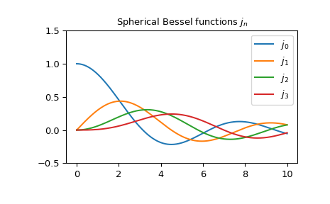
前几个带有实数参数的 \(j_n\)
>>> import matplotlib.pyplot as plt
>>> x = np.arange(0.0, 10.0, 0.01)
>>> fig, ax = plt.subplots()
>>> ax.set_ylim(-0.5, 1.5)
>>> ax.set_title(r'Spherical Bessel functions $j_n$')
>>> for n in np.arange(0, 4):
...     ax.plot(x, spherical_jn(n, x), label=rf'$j_{n}$')
>>> plt.legend(loc='best')
>>> plt.show()