scipy.signal.ShortTimeFFT.
extent#
- ShortTimeFFT.extent(n, axes_seq='tf', center_bins=False)[source]#
返回最小和最大的时间-频率值。
返回一个包含四个浮点数的元组
(t0, t1, f0, f1),对于 'tf' 和(f0, f1, t0, t1)对于 'ft',描述了stft的时频域的角。该元组可以作为具有相同名称的参数传递给matplotlib.pyplot.imshow。- 参数:
- nint
输入信号中的样本数。
- axes_seq{‘tf’, ‘ft’}
先返回时间范围,然后返回频率范围,反之亦然。
- center_bins: bool
如果设置(默认
False),则时间槽和频率箱的值将从侧面移动到中间。 当将stft值绘制为阶跃函数时(即没有插值),这很有用。
参见
matplotlib.pyplot.imshow将数据显示为图像。
scipy.signal.ShortTimeFFT此方法所属的类。
示例
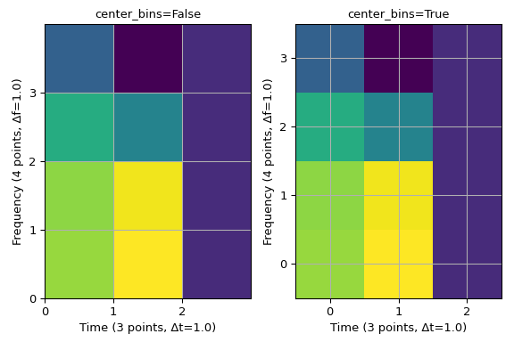
以下两个图说明了参数 center_bins 的效果:网格线表示 STFT 的三个时间和四个频率值。 左图,其中
(t0, t1, f0, f1) = (0, 3, 0, 4)作为参数extent传递给imshow,显示了时间和频率值位于相应箱的下边缘的标准行为。 右图,其中(t0, t1, f0, f1) = (-0.5, 2.5, -0.5, 3.5),显示了在传递center_bins=True时,箱位于各自值的中心。>>> import matplotlib.pyplot as plt >>> import numpy as np >>> from scipy.signal import ShortTimeFFT ... >>> n, m = 12, 6 >>> SFT = ShortTimeFFT.from_window('hann', fs=m, nperseg=m, noverlap=0) >>> Sxx = SFT.stft(np.cos(np.arange(n))) # produces a colorful plot ... >>> fig, axx = plt.subplots(1, 2, tight_layout=True, figsize=(6., 4.)) >>> for ax_, center_bins in zip(axx, (False, True)): ... ax_.imshow(abs(Sxx), origin='lower', interpolation=None, aspect='equal', ... cmap='viridis', extent=SFT.extent(n, 'tf', center_bins)) ... ax_.set_title(f"{center_bins=}") ... ax_.set_xlabel(f"Time ({SFT.p_num(n)} points, Δt={SFT.delta_t})") ... ax_.set_ylabel(f"Frequency ({SFT.f_pts} points, Δf={SFT.delta_f})") ... ax_.set_xticks(SFT.t(n)) # vertical grid line are timestamps ... ax_.set_yticks(SFT.f) # horizontal grid line are frequency values ... ax_.grid(True) >>> plt.show()
请注意,具有恒定颜色的阶跃式行为是由将
interpolation=None传递给imshow引起的。