scipy.special.eval_legendre#

scipy.special.eval_legendre(n, x, out=None) = <ufunc 'eval_legendre'>#

在某点评估勒让德多项式。

勒让德多项式可以通过高斯超几何函数 \({}_2F_1\) 定义为

\[P_n(x) = {}_2F_1(-n, n + 1; 1; (1 - x)/2).\]

当 \(n\) 是整数时，结果是次数为 \(n\) 的多项式。有关详细信息，请参阅 [AS] (或等效地 [DLMF]) 的 22.5.49。

参数:

返回:

另请参阅

参考文献

[AS]

Milton Abramowitz 和 Irene A. Stegun 编. 带有公式、图表和数学表格的数学函数手册。纽约：Dover，1972。

NIST 数学函数数字图书馆，https://dlmf.nist.gov/15.9.E7

示例

>>> import numpy as np
>>> from scipy.special import eval_legendre

评估零阶勒让德多项式在 x = 0 处的值

>>> eval_legendre(0, 0)
1.0

评估一阶勒让德多项式在 -1 到 1 之间的值

>>> X = np.linspace(-1, 1, 5)  # Domain of Legendre polynomials
>>> eval_legendre(1, X)
array([-1. , -0.5,  0. ,  0.5,  1. ])

评估 0 到 4 阶勒让德多项式在 x = 0 处的值

>>> N = range(0, 5)
>>> eval_legendre(N, 0)
array([ 1.   ,  0.   , -0.5  ,  0.   ,  0.375])

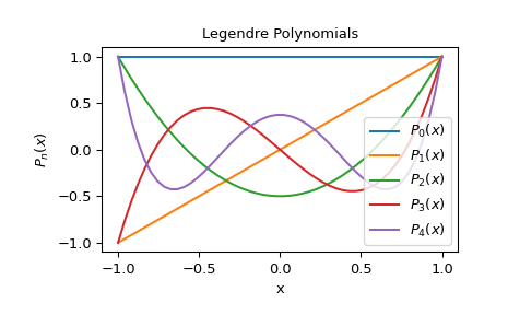
绘制 0 到 4 阶勒让德多项式

>>> X = np.linspace(-1, 1)

>>> import matplotlib.pyplot as plt
>>> for n in range(0, 5):
...     y = eval_legendre(n, X)
...     plt.plot(X, y, label=r'$P_{}(x)$'.format(n))

>>> plt.title("Legendre Polynomials")
>>> plt.xlabel("x")
>>> plt.ylabel(r'$P_n(x)$')
>>> plt.legend(loc='lower right')
>>> plt.show()