scipy.spatial.

SphericalVoronoi

class scipy.spatial.SphericalVoronoi(points, radius=1, center=None, threshold=1e-06)

球面上的 Voronoi 图。

0.18.0 版新增。

参数:

points浮点型 ndarray，形状为 (npoints, ndim)

用于构建球面 Voronoi 图的点的坐标。

radius浮点型，可选

球体的半径（默认值：1）

center浮点型 ndarray，形状为 (ndim,)

球体中心（默认值：原点）

threshold浮点型

用于检测重复点以及点与球体参数之间不匹配的阈值。（默认值：1e-06）

属性:

points双精度数组，形状为 (npoints, ndim)

用于生成 Voronoi 图的 ndim 维点

radius双精度

球体半径

center双精度数组，形状为 (ndim,)

球体中心

vertices双精度数组，形状为 (nvertices, ndim)

对应于点的 Voronoi 顶点

regions整数列表的列表，形状为 (npoints, _ )

第 n 个条目是一个列表，包含属于 points 中第 n 个点的顶点的索引

方法

calculate_areas()

计算 Voronoi 区域的面积。

抛出:

ValueError

如果 points 中存在重复项。如果提供的 radius 与 points 不一致。

另请参阅

Voronoi

N 维常规 Voronoi 图。

备注

球面 Voronoi 图算法的步骤如下：计算输入点（生成器）的凸包，这等同于它们在球体表面上的 Delaunay 三角剖分 [Caroli]。然后使用凸包邻域信息来围绕每个生成器对 Voronoi 区域顶点进行排序。后一种方法比基于角度的 Voronoi 区域顶点排序方法对浮点问题的影响要小得多。

对球面 Voronoi 算法性能的实证评估表明其时间复杂度为二次方（对数线性是最佳的，但算法实现更具挑战性）。

参考文献

[Caroli]

Caroli 等人。球体上或接近球体点的稳健高效 Delaunay 三角剖分。研究报告 RR-7004, 2009。

[VanOosterom]

Van Oosterom 和 Strackee。《平面三角形的立体角》。IEEE 生物医学工程汇刊，2，1983，第 125–126 页。

示例

在浏览器中试试！

导入一些模块并在立方体上取一些点

>>> import numpy as np
>>> import matplotlib.pyplot as plt
>>> from scipy.spatial import SphericalVoronoi, geometric_slerp
>>> from mpl_toolkits.mplot3d import proj3d
>>> # set input data
>>> points = np.array([[0, 0, 1], [0, 0, -1], [1, 0, 0],
...                    [0, 1, 0], [0, -1, 0], [-1, 0, 0], ])

计算球面 Voronoi 图

>>> radius = 1
>>> center = np.array([0, 0, 0])
>>> sv = SphericalVoronoi(points, radius, center)

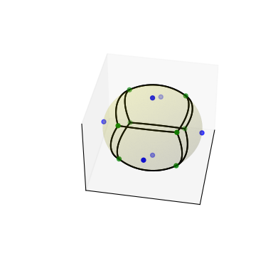
生成图表

>>> # sort vertices (optional, helpful for plotting)
>>> sv.sort_vertices_of_regions()
>>> t_vals = np.linspace(0, 1, 2000)
>>> fig = plt.figure()
>>> ax = fig.add_subplot(111, projection='3d')
>>> # plot the unit sphere for reference (optional)
>>> u = np.linspace(0, 2 * np.pi, 100)
>>> v = np.linspace(0, np.pi, 100)
>>> x = np.outer(np.cos(u), np.sin(v))
>>> y = np.outer(np.sin(u), np.sin(v))
>>> z = np.outer(np.ones(np.size(u)), np.cos(v))
>>> ax.plot_surface(x, y, z, color='y', alpha=0.1)
>>> # plot generator points
>>> ax.scatter(points[:, 0], points[:, 1], points[:, 2], c='b')
>>> # plot Voronoi vertices
>>> ax.scatter(sv.vertices[:, 0], sv.vertices[:, 1], sv.vertices[:, 2],
...                    c='g')
>>> # indicate Voronoi regions (as Euclidean polygons)
>>> for region in sv.regions:
...    n = len(region)
...    for i in range(n):
...        start = sv.vertices[region][i]
...        end = sv.vertices[region][(i + 1) % n]
...        result = geometric_slerp(start, end, t_vals)
...        ax.plot(result[..., 0],
...                result[..., 1],
...                result[..., 2],
...                c='k')
>>> ax.azim = 10
>>> ax.elev = 40
>>> _ = ax.set_xticks([])
>>> _ = ax.set_yticks([])
>>> _ = ax.set_zticks([])
>>> fig.set_size_inches(4, 4)
>>> plt.show()

返回在新标签页中打开