percentile_filter#
- scipy.ndimage.percentile_filter(input, percentile, size=None, footprint=None, output=None, mode='reflect', cval=0.0, origin=0, *, axes=None)[source]#
计算多维百分位数滤波器。
- 参数:
- inputarray_like
输入数组。
- percentilescalar
百分位数参数可以小于零,例如,percentile = -20 等同于 percentile = 80
- size标量或元组,可选
参见下面的 footprint。如果指定了 footprint,则忽略。
- footprint数组,可选
size 或 footprint 必须定义其中一个。size 定义了从输入数组的每个元素位置获取的形状,用于定义滤波器函数的输入。footprint 是一个布尔数组,它(隐式地)指定了一个形状,并且还指定了该形状中哪些元素将传递给滤波器函数。因此
size=(n,m)等效于footprint=np.ones((n,m))。我们会根据输入数组的维度数调整 size,因此如果输入数组的形状是 (10,10,10),并且 size 是 2,则实际使用的尺寸是 (2,2,2)。当指定 footprint 时,size 将被忽略。- output数组或 dtype,可选
用于放置输出的数组,或返回数组的 dtype。默认情况下,将创建一个与 input 具有相同 dtype 的数组。
- mode{‘reflect’, ‘constant’, ‘nearest’, ‘mirror’, ‘wrap’},可选
参数 mode 决定了输入数组如何在其边界之外进行扩展。默认值为 ‘reflect’。每个有效值的行为如下:
- ‘reflect’ (d c b a | a b c d | d c b a)
通过最后一个像素的边缘反射来扩展输入。此模式有时也称为半样本对称。
- ‘constant’ (k k k k | a b c d | k k k k)
通过用相同的常数值(由 cval 参数定义)填充超出边缘的所有值来扩展输入。
- ‘nearest’ (a a a a | a b c d | d d d d)
通过复制最后一个像素来扩展输入。
- ‘mirror’ (d c b | a b c d | c b a)
通过最后一个像素的中心反射来扩展输入。此模式有时也称为全样本对称。
- ‘wrap’ (a b c d | a b c d | a b c d)
通过环绕到对边来扩展输入。
为了与插值函数保持一致,也可以使用以下模式名称:
- ‘grid-mirror’
这是 ‘reflect’ 的同义词。
- ‘grid-constant’
这是 ‘constant’ 的同义词。
- ‘grid-wrap’
这是 ‘wrap’ 的同义词。
- cval标量,可选
如果 mode 为 ‘constant’,用于填充输入边缘之外的值。默认值为 0.0。
- origin整数或序列,可选
控制滤波器在输入数组像素上的位置。值为 0(默认值)将滤波器居中于像素,正值将滤波器向左移动,负值则向右移动。通过传入一个长度等于输入数组维度数的 origin 序列,可以在每个轴上指定不同的位移。
- axes整数元组或 None,可选
如果为 None,则 input 将沿所有轴进行过滤。否则,input 将沿指定的轴进行过滤。当指定 axes 时,用于 size、origin 和/或 mode 的任何元组必须与 axes 的长度匹配。这些元组中的第 i 个条目对应于 axes 中的第 i 个条目。
- 返回值:
- percentile_filterndarray
过滤后的数组。与 input 具有相同的形状。
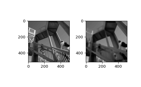
示例
>>> from scipy import ndimage, datasets
>>> import matplotlib.pyplot as plt
>>> fig = plt.figure()
>>> plt.gray()  # show the filtered result in grayscale
>>> ax1 = fig.add_subplot(121)  # left side
>>> ax2 = fig.add_subplot(122)  # right side
>>> ascent = datasets.ascent()
>>> result = ndimage.percentile_filter(ascent, percentile=20, size=20)
>>> ax1.imshow(ascent)
>>> ax2.imshow(result)
>>> plt.show()