Shapiro-Wilk 正态性检验#
假设我们希望根据测量结果推断一项医学研究中成年男性的体重是否不符合正态分布 [1]。体重(磅)记录在下面的数组 x 中。
import numpy as np
x = np.array([148, 154, 158, 160, 161, 162, 166, 170, 182, 195, 236])
正态性检验 scipy.stats.shapiro [1] 和 [2] 首先根据观测值与正态分布预期次序统计量之间的关系计算一个统计量。
from scipy import stats
res = stats.shapiro(x)
res.statistic
np.float64(0.7888146948631716)
从正态分布中抽取的样本,该统计量的值趋于较高(接近 1)。
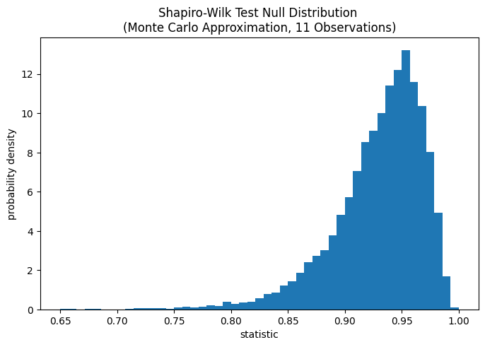
该测试通过将统计量的观测值与零分布(null distribution)进行比较来执行:零分布是指在零假设(即体重数据来自正态分布)下形成的统计量值的分布。对于此正态性检验,零分布不易精确计算,因此通常通过蒙特卡洛方法(即从正态分布中抽取与 x 相同大小的多个样本,并计算每个样本的统计量值)进行近似。
def statistic(x):
    # Get only the `shapiro` statistic; ignore its p-value
    return stats.shapiro(x).statistic
ref = stats.monte_carlo_test(x, stats.norm.rvs, statistic,
                             alternative='less')
import matplotlib.pyplot as plt
fig, ax = plt.subplots(figsize=(8, 5))
bins = np.linspace(0.65, 1, 50)

def plot(ax):  # we'll reuse this
    ax.hist(ref.null_distribution, density=True, bins=bins)
    ax.set_title("Shapiro-Wilk Test Null Distribution \n"
                 "(Monte Carlo Approximation, 11 Observations)")
    ax.set_xlabel("statistic")
    ax.set_ylabel("probability density")

plot(ax)
plt.show()
这种比较通过 P 值量化:P 值是零分布中小于或等于统计量观测值的比例。
fig, ax = plt.subplots(figsize=(8, 5))
plot(ax)
annotation = (f'p-value={res.pvalue:.6f}\n(highlighted area)')
props = dict(facecolor='black', width=1, headwidth=5, headlength=8)
_ = ax.annotate(annotation, (0.75, 0.1), (0.68, 0.7), arrowprops=props)
i_extreme = np.where(bins <= res.statistic)[0]
for i in i_extreme:
    ax.patches[i].set_color('C1')
plt.xlim(0.65, 0.9)
plt.ylim(0, 4)
plt.show()
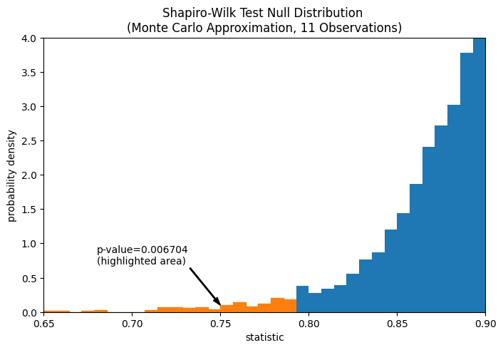
res.pvalue
np.float64(0.006703814061898823)
如果 P 值“很小”——也就是说,从正态分布总体中抽取数据产生如此极端的统计量值的概率很低——这可以作为反对零假设的证据,支持备择假设:体重数据并非来自正态分布。请注意,
反之则不成立;也就是说,该测试不用于提供支持零假设的证据。
将哪些值视为“小”的阈值应在数据分析之前确定 [3],并考虑假阳性(错误地拒绝零假设)和假阴性(未能拒绝错误的零假设)的风险。