皮尔逊相关系数#
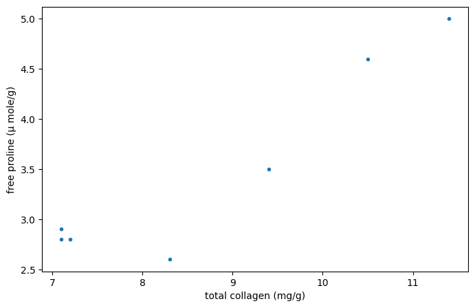
考虑来自 [1] 的以下数据,该研究调查了不健康人肝脏中游离脯氨酸(一种氨基酸)与总胶原蛋白(一种常存在于结缔组织中的蛋白质)之间的关系。
下面的 x 和 y 数组记录了这两种化合物的测量值。这些观测值是配对的:每个游离脯氨酸的测量值都与相同索引处的总胶原蛋白测量值来自同一肝脏。
import numpy as np
# total collagen (mg/g dry weight of liver)
x = np.array([7.1, 7.1, 7.2, 8.3, 9.4, 10.5, 11.4])
# free proline (μ mole/g dry weight of liver)
y = np.array([2.8, 2.9, 2.8, 2.6, 3.5, 4.6, 5.0])
import matplotlib.pyplot as plt
fig, ax = plt.subplots(figsize=(8, 5))
ax.plot(x, y, '.')
ax.set_xlabel("total collagen (mg/g)")
ax.set_ylabel("free proline (μ mole/g)")
plt.show()
这些数据在 [2] 中使用 Spearman 相关系数进行了分析,该统计量对样本之间的单调相关性敏感。在这里,我们将使用皮尔逊相关系数({class}scipy.stats.pearsonr`)分析数据,该系数对线性相关性敏感。
from scipy import stats
res = stats.pearsonr(x, y)
res.statistic
np.float64(0.9347467974524514)
对于具有强正线性相关的样本,该统计量的值趋于高(接近 1);对于具有强负线性相关的样本,其值趋于低(接近 -1);对于线性相关性弱的样本,其值幅值小(接近零)。
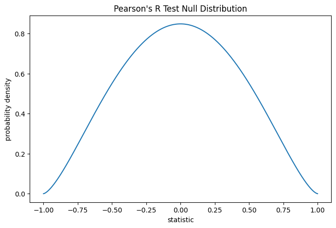
通过将统计量的观测值与零分布进行比较来执行检验:零分布是在总胶原蛋白和游离脯氨酸测量值来自独立正态分布的零假设下得出的统计量值的分布。
在零假设下,总体相关系数为零,样本相关系数遵循区间 \((-1, 1)\) 上的 Beta 分布,形状参数为 \(a = b = \frac{n}{2}-1\),其中 \(n\) 是每个样本中的观测值数量。
n = len(x)  # len(x) == len(y)
a = b = n/2 - 1  # shape parameter
loc, scale = -1, 2  # support is (-1, 1)
dist = stats.beta(a=a, b=b, loc=loc, scale=scale)
r_vals = np.linspace(-1, 1, 1000)
pdf = dist.pdf(r_vals)
fig, ax = plt.subplots(figsize=(8, 5))
def plot(ax):  # we'll re-use this
    ax.plot(r_vals, pdf)
    ax.set_title("Pearson's R Test Null Distribution")
    ax.set_xlabel("statistic")
    ax.set_ylabel("probability density")
plot(ax)
plt.show()
比较通过 p 值量化:零分布中与统计量观测值一样极端或更极端的值的比例。在统计量为正的双侧检验中,零分布中大于变换后统计量的值和小于观测统计量负值的值都被认为是“更极端”的。
fig, ax = plt.subplots(figsize=(8, 5))
plot(ax)
rs = res.statistic  # original statistic
pvalue = dist.cdf(-rs) + dist.sf(rs)
annotation = (f'p-value={pvalue:.4f}\n(shaded area)')
props = dict(facecolor='black', width=1, headwidth=5, headlength=8)
_ = ax.annotate(annotation, (rs, 0.01), (0.25, 0.1), arrowprops=props)
i = r_vals >= rs
ax.fill_between(r_vals[i], y1=0, y2=pdf[i], color='C0')
i = r_vals <= -rs
ax.fill_between(r_vals[i], y1=0, y2=pdf[i], color='C0')
ax.set_xlim(-1.1, 1.1)
ax.set_ylim(0, 0.9)
plt.show()
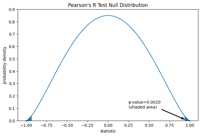
res.pvalue # two-sided p-value
np.float64(0.002016532795489407)
如果 p 值“小”——也就是说,从独立正态分布中抽样数据产生如此极端统计量值的概率很低——这可以作为反对零假设的证据,转而支持备择假设:总胶原蛋白和游离脯氨酸的分布不是独立的。请注意,
反之则不然;也就是说,该检验不用于提供支持零假设的证据。
“小”值的阈值应在分析数据之前做出选择 [3],并考虑假阳性(错误地拒绝零假设)和假阴性(未能拒绝错误的零假设)的风险。
小的 p 值并非大效应的证据;相反,它们只能提供“显著”效应的证据,这意味着它们在零假设下不太可能发生。
假设在进行实验之前,作者有理由预测总胶原蛋白和游离脯氨酸测量之间存在正线性相关,并且他们选择通过单侧备择假设来评估零假设的合理性:游离脯氨酸与总胶原蛋白呈正线性相关。在这种情况下,只有零分布中大于或等于观测统计量的值才会被认为是更极端的。
res = stats.pearsonr(x, y, alternative='greater')
res.statistic
fig, ax = plt.subplots(figsize=(8, 5))
plot(ax)
pvalue = dist.sf(rs)
annotation = (f'p-value={pvalue:.6f}\n(shaded area)')
props = dict(facecolor='black', width=1, headwidth=5, headlength=8)
_ = ax.annotate(annotation, (rs, 0.01), (0.86, 0.04), arrowprops=props)
i = r_vals >= rs
ax.fill_between(r_vals[i], y1=0, y2=pdf[i], color='C0')
ax.set_xlim(0.85, 1)
ax.set_ylim(0, 0.1)
plt.show()
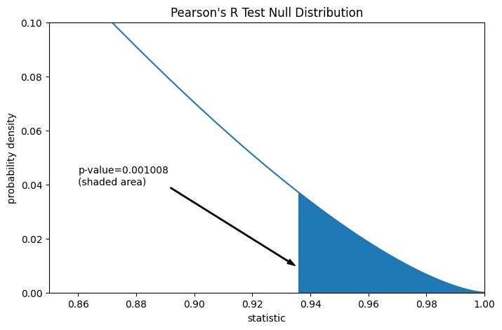
res.pvalue # one-sided p-value; half of the two-sided p-value
np.float64(0.0010082663977447036)
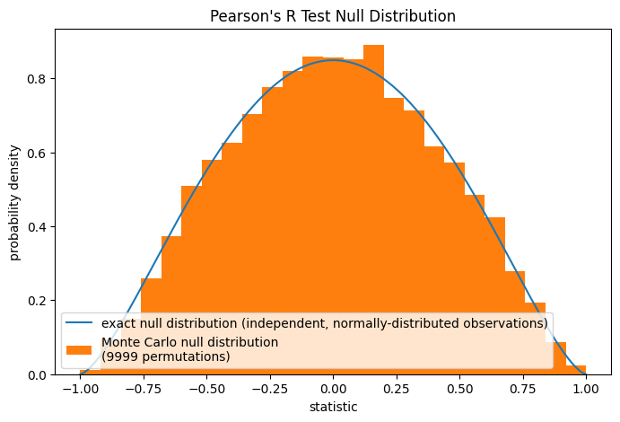
请注意,Beta 分布是此零假设下任何大小样本的精确零分布。我们可以通过计算蒙特卡洛零分布来验证这一点:明确地从独立的正常分布中抽取样本,并计算每对的皮尔逊统计量。
rng = np.random.default_rng(332520619051409741187796892627751113442)

def statistic(x, y, axis):
    return stats.pearsonr(x, y, axis=axis).statistic  # ignore pvalue

ref = stats.monte_carlo_test((x, y), rvs=(rng.standard_normal, rng.standard_normal),
                             statistic=statistic, alternative='greater', n_resamples=9999)

fig, ax = plt.subplots(figsize=(8, 5))
plot(ax)
ax.hist(ref.null_distribution, np.linspace(-1, 1, 26), density=True)
ax.legend(['exact null distribution (independent, normally-distributed observations)',
           f'Monte Carlo null distribution \n({len(ref.null_distribution)} permutations)'])
plt.show()
这通常是一个合理的零假设来检验,但在其他情况下,进行置换检验可能更合适:在总胶原蛋白和游离脯氨酸独立的零假设下(但不一定正态分布),每个游离脯氨酸测量值与任何总胶原蛋白测量值被观测到的可能性是均等的。因此,我们可以通过计算 x 和 y 之间每个可能的元素配对下的统计量来形成精确的零分布。当我们为 pearsonr 提供 method=stats.PermutationMethod() 时,使用的就是这种零分布。
res = stats.pearsonr(x, y, alternative='greater', method=stats.PermutationMethod())
res.pvalue
np.float64(0.005555555555555556)