偏度检验#
此函数检验的零假设是:样本所来自总体的偏度与对应正态分布的偏度相同。
假设我们希望根据测量结果推断,医学研究中成年男性体重是否不呈正态分布[1]。体重(磅)记录在下面的数组x中。
import numpy as np
x = np.array([148, 154, 158, 160, 161, 162, 166, 170, 182, 195, 236])
偏度检验scipy.stats.skewtest(来自[2])首先计算一个基于样本偏度的统计量。
from scipy import stats
res = stats.skewtest(x)
res.statistic
np.float64(2.7788579769903414)
由于正态分布的偏度为零,因此从正态分布中抽取的样本的此统计量的大小倾向于较低。
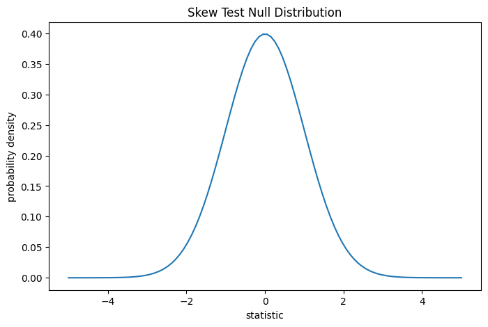
通过将统计量的观测值与零分布进行比较来执行检验:零分布是在体重从正态分布中抽取的零假设下得到的统计量值分布。
对于此检验,对于非常大的样本,统计量的零分布是标准正态分布。
import matplotlib.pyplot as plt
dist = stats.norm()
st_val = np.linspace(-5, 5, 100)
pdf = dist.pdf(st_val)
fig, ax = plt.subplots(figsize=(8, 5))

def st_plot(ax):  # we'll reuse this
    ax.plot(st_val, pdf)
    ax.set_title("Skew Test Null Distribution")
    ax.set_xlabel("statistic")
    ax.set_ylabel("probability density")

st_plot(ax)
plt.show()
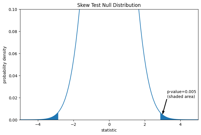
这种比较通过 p 值进行量化:p 值是零分布中与观测到的统计量值一样极端或更极端的值的比例。在双侧检验中,零分布中大于观测统计量的元素和小于观测统计量负值的元素都被认为是“更极端”。
fig, ax = plt.subplots(figsize=(8, 5))
st_plot(ax)
pvalue = dist.cdf(-res.statistic) + dist.sf(res.statistic)
annotation = (f'p-value={pvalue:.3f}\n(shaded area)')
props = dict(facecolor='black', width=1, headwidth=5, headlength=8)
_ = ax.annotate(annotation, (3, 0.005), (3.25, 0.02), arrowprops=props)
i = st_val >= res.statistic
ax.fill_between(st_val[i], y1=0, y2=pdf[i], color='C0')
i = st_val <= -res.statistic
ax.fill_between(st_val[i], y1=0, y2=pdf[i], color='C0')
ax.set_xlim(-5, 5)
ax.set_ylim(0, 0.1)
plt.show()
res.pvalue
np.float64(0.005455036974740185)
如果 p 值“很小”——也就是说,从正态分布总体中抽样数据产生如此极端的统计量值的概率很低——这可以作为反对零假设的证据,转而支持备择假设:体重并非来自正态分布。请注意
反之则不成立;也就是说,此检验不能用于提供支持零假设的证据。
“小”值的阈值应在分析数据之前做出选择[3],并考虑假阳性(错误地拒绝零假设)和假阴性(未能拒绝错误的零假设)的风险。
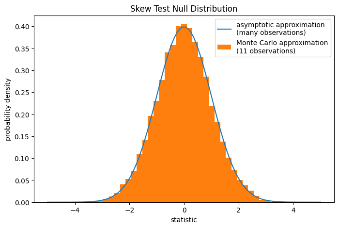
请注意,标准正态分布提供了零分布的渐近近似;它仅对于具有大量观测值的样本准确。对于像我们这样的小样本,scipy.stats.monte_carlo_test 可能会提供更准确(尽管是随机的)的精确 p 值近似。
def statistic(x, axis):
    # get just the skewtest statistic; ignore the p-value
    return stats.skewtest(x, axis=axis).statistic

res = stats.monte_carlo_test(x, stats.norm.rvs, statistic)
fig, ax = plt.subplots(figsize=(8, 5))
st_plot(ax)
ax.hist(res.null_distribution, np.linspace(-5, 5, 50),
        density=True)
ax.legend(['asymptotic approximation\n(many observations)',
           'Monte Carlo approximation\n(11 observations)'])
plt.show()
res.pvalue
np.float64(0.005)
在这种情况下,即使对于我们的小样本,渐近近似和蒙特卡洛近似也相当接近。