Jarque-Bera 拟合优度检验#
假设我们希望根据测量结果推断医疗研究中成年男性体重是否不呈正态分布 [1]。体重(磅)记录在下面的数组 x 中。
import numpy as np
x = np.array([148, 154, 158, 160, 161, 162, 166, 170, 182, 195, 236])
Jarque-Bera 检验 scipy.stats.jarque_bera 首先根据样本偏度和峰度计算一个统计量。
from scipy import stats
res = stats.jarque_bera(x)
res.statistic
np.float64(6.982848237344646)
由于正态分布的偏度为零,峰度(“超额”或“费舍尔”峰度)也为零,因此从正态分布中抽取的样本的该统计量值往往较低。
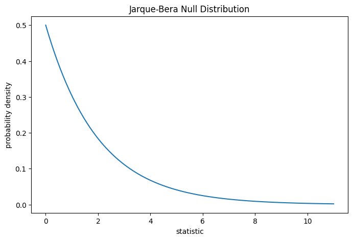
通过将观察到的统计量值与零分布进行比较来执行检验:零分布是在零假设(即体重是从正态分布中抽取的)下得出的统计量值的分布。
对于 Jarque-Bera 检验,对于非常大的样本,零分布是具有两个自由度的卡方分布。
import matplotlib.pyplot as plt

dist = stats.chi2(df=2)
jb_val = np.linspace(0, 11, 100)
pdf = dist.pdf(jb_val)
fig, ax = plt.subplots(figsize=(8, 5))

def jb_plot(ax):  # we'll reuse this
    ax.plot(jb_val, pdf)
    ax.set_title("Jarque-Bera Null Distribution")
    ax.set_xlabel("statistic")
    ax.set_ylabel("probability density")

jb_plot(ax)
plt.show();
比较通过 p 值量化:零分布中大于或等于观察到的统计量值的比例。
fig, ax = plt.subplots(figsize=(8, 5))
jb_plot(ax)
pvalue = dist.sf(res.statistic)
annotation = (f'p-value={pvalue:.6f}\n(shaded area)')
props = dict(facecolor='black', width=1, headwidth=5, headlength=8)
_ = ax.annotate(annotation, (7.5, 0.01), (8, 0.05), arrowprops=props)
i = jb_val >= res.statistic  # indices of more extreme statistic values
ax.fill_between(jb_val[i], y1=0, y2=pdf[i])
ax.set_xlim(0, 11)
ax.set_ylim(0, 0.3)
plt.show()
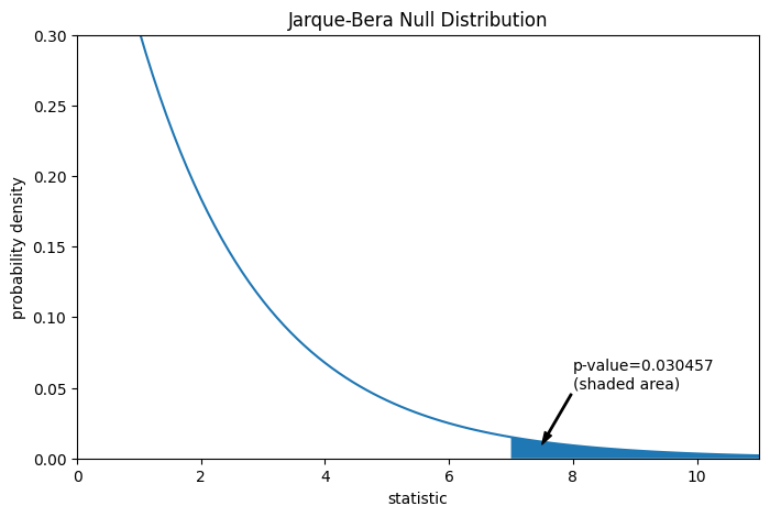
res.pvalue
np.float64(0.03045746622458189)
如果 p 值“很小”——也就是说,如果从正态分布总体中抽取数据,产生如此极端的统计量值的概率很低——这可以作为反对零假设,支持备择假设的证据:体重不是从正态分布中抽取的。请注意
反之则不然;也就是说,该检验不用于为零假设提供证据。
将“小”值视为阈值的选择应在数据分析之前进行 [2],并考虑假阳性(错误地拒绝零假设)和假阴性(未能拒绝错误的零假设)的风险。
请注意,卡方分布提供了零分布的渐近近似;它仅对具有许多观测值的样本准确。对于像我们这样的小样本,scipy.stats.monte_carlo_test 可以提供更准确(尽管是随机的)的精确 p 值近似。
def statistic(x, axis):
    # underlying calculation of the Jarque Bera statistic
    s = stats.skew(x, axis=axis)
    k = stats.kurtosis(x, axis=axis)
    return x.shape[axis]/6 * (s**2 + k**2/4)

res = stats.monte_carlo_test(x, stats.norm.rvs, statistic,
                             alternative='greater')
fig, ax = plt.subplots(figsize=(8, 5))
jb_plot(ax)
ax.hist(res.null_distribution, np.linspace(0, 10, 50),
        density=True)
ax.legend(['asymptotic approximation (many observations)',
           'Monte Carlo approximation (11 observations)'])
plt.show()
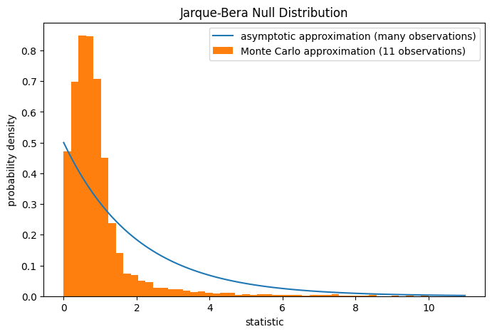
res.pvalue
np.float64(0.0095)
此外,尽管它们的随机性,以这种方式计算的 p 值可以精确控制零假设的错误拒绝率 [3]。