SciPy 中的通用非均匀随机数采样

SciPy 提供了一个接口，可以访问许多通用非均匀随机数生成器，以从各种单变量连续和离散分布中采样随机变量。快速 C 库 UNU.RAN 的实现用于提高速度和性能。请查看 UNU.RAN 的文档，以深入了解这些方法。本教程和所有生成器的文档都大量参考了它。

简介

随机变量生成是一个小的研究领域，它处理从各种分布生成随机变量的算法。通常假设可以使用均匀随机数生成器。这是一个程序，它产生一系列独立且同分布的连续 U(0,1) 随机变量（即 (0,1) 区间上的均匀随机变量）。当然，现实世界中的计算机永远无法生成理想的随机数，也无法生成任意精度的数字，但最先进的均匀随机数生成器接近于这个目标。因此，随机变量生成处理将这样的 U(0,1) 随机数序列转换为非均匀随机变量的问题。这些方法是通用的，并且以黑盒方式工作。

一些实现此目的的方法是

• 反演方法：当累积分布函数的逆 \(F^{-1}\) 已知时，随机变量生成很容易。我们只需生成一个均匀分布的 U(0,1) 随机数 U，然后返回 \(X = F^{-1}(U)\)。由于逆的闭合形式解很少见，因此通常需要依赖于逆的近似值（例如 ndtri，stdtrit）。通常，特殊函数的实现比 UNU.RAN 中的反演方法慢得多。

• 拒绝采样法：拒绝采样法，也称为接受-拒绝采样法，由约翰·冯·诺依曼于 1951 年提出 [1]。它涉及计算 PDF 的上限（也称为帽子函数），并使用反演方法从该上限生成一个随机变量，例如 Y。然后，可以在 0 到 Y 处上限的值之间绘制一个均匀随机数。如果此数字小于 Y 处的 PDF，则返回样本，否则拒绝它。请参阅 TransformedDensityRejection。

• 均匀比法：这是一种接受-拒绝采样法，它使用最小边界矩形来构建帽子函数。请参阅 scipy.stats.rvs_ratio_uniforms。

• 离散分布的反演：与连续情况相比，区别在于 \(F\) 现在是一个阶梯函数。为了在计算机中实现这一点，使用了搜索算法，最简单的是顺序搜索。从 U(0, 1) 生成一个均匀随机数，并对概率进行求和，直到累积概率超过均匀随机数。发生这种情况的索引是所需的随机变量，并被返回。

有关这些算法的更多详细信息，请参阅 UNU.RAN 用户手册的附录。

在生成分布的随机变量时，有两个因素决定了生成器的速度：设置步骤和实际采样。根据情况，不同的生成器可能是最佳的。例如，如果需要从具有固定形状参数的给定分布中重复抽取大量样本，则如果采样速度快，则缓慢的设置是可以接受的。这称为固定参数情况。如果目标是为不同的形状参数生成分布的样本（变化参数情况），则需要为每个参数重复执行的昂贵设置会导致非常差的性能。在这种情况下，快速设置对于实现良好的性能至关重要。下表概述了不同方法的设置和采样速度。

连续分布的方法	必需输入	可选输入	设置速度	采样速度
变换密度拒绝	pdf，dpdf	无	慢	快
数值逆厄米特	cdf	pdf，dpdf	（非常）慢	（非常）快
数值逆多项式	pdf	cdf	（非常）慢	（非常）快
简单比率均匀	pdf	无	快	慢

其中

• pdf：概率密度函数

• dpdf：pdf 的导数

• cdf：累积分布函数

要将数值反演方法 NumericalInversePolynomial 应用于 SciPy 中的大量连续分布，且工作量最小，请查看 scipy.stats.sampling.FastGeneratorInversion.

离散分布的方法	必需输入	可选输入	设置速度	采样速度
离散别名瓮	pv	pmf	慢	非常快
离散引导表	pv	pmf	慢	非常快

其中

• pv：概率向量

• pmf：概率质量函数

有关 UNU.RAN 中实现的生成器的更多详细信息，请参阅 [2] 和 [3].

接口的基本概念

每个生成器都需要在开始从中采样之前进行设置。这可以通过实例化该类的对象来完成。大多数生成器都以分布对象作为输入，该对象包含所需方法（如 PDF、CDF 等）的实现。除了分布对象之外，还可以传递用于设置生成器的参数。也可以使用 domain 参数截断分布。所有生成器都需要一个均匀随机数流，这些随机数流被转换为给定分布的随机变量。这是通过传递一个 random_state 参数来完成的，该参数使用 NumPy BitGenerator 作为均匀随机数生成器。 random_state 可以是整数、numpy.random.Generator 或 numpy.random.RandomState.

警告

不建议使用 NumPy < 1.19.0，因为它没有用于生成均匀随机数的快速 Cython API，对于实际使用来说可能太慢。

所有生成器都有一个通用的 rvs 方法，可用于从给定分布中抽取样本。

下面显示了此接口的示例

>>> from scipy.stats.sampling import TransformedDensityRejection
>>> from math import exp
>>>
>>> class StandardNormal:
...     def pdf(self, x: float) -> float:
...         # note that the normalization constant isn't required
...         return exp(-0.5 * x*x)
...     def dpdf(self, x: float) -> float:
...         return -x * exp(-0.5 * x*x)
...
>>> dist = StandardNormal()
>>>
>>> urng = np.random.default_rng()
>>> rng = TransformedDensityRejection(dist, random_state=urng)

如示例所示，我们首先初始化一个分布对象，其中包含生成器所需方法的实现。在本例中，我们使用 TransformedDensityRejection (TDR) 方法，该方法需要一个 PDF 及其关于 x（即变量）的导数。

注意

请注意，分布的方法（即 pdf、dpdf 等）不需要向量化。它们应该接受和返回浮点数。

注意

也可以将 SciPy 分布作为参数传递。但是，请注意，该对象并不总是包含某些生成器所需的所有信息，例如 TDR 方法的 PDF 导数。依赖 SciPy 分布也可能会降低性能，因为方法（如 pdf 和 cdf）的向量化。在这两种情况下，都可以实现一个自定义分布对象，该对象包含所有必需的方法，并且如上例所示，该对象不是向量化的。如果要将数值反演方法应用于 SciPy 中定义的分布，请查看 scipy.stats.sampling.FastGeneratorInversion。

在上面的例子中，我们已经设置了一个TransformedDensityRejection方法的对象，用于从标准正态分布中采样。现在，我们可以通过调用rvs方法开始从我们的分布中采样。

>>> rng.rvs()
-1.526829048388144
>>> rng.rvs((5, 3))
array([[ 2.06206883,  0.15205036,  1.11587367],
       [-0.30775562,  0.29879802, -0.61858268],
       [-1.01049115,  0.78853694, -0.23060766],
       [-0.60954752,  0.29071797, -0.57167182],
       [ 0.9331694 , -0.95605208,  1.72195199]])

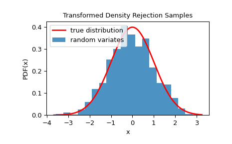
我们还可以通过可视化样本的直方图来检查样本是否是从正确的分布中抽取的。

>>> import matplotlib.pyplot as plt
>>> from scipy.stats import norm
>>> from scipy.stats.sampling import TransformedDensityRejection
>>> from math import exp
>>>
>>> class StandardNormal:
...     def pdf(self, x: float) -> float:
...         # note that the normalization constant isn't required
...         return exp(-0.5 * x*x)
...     def dpdf(self, x: float) -> float:
...         return -x * exp(-0.5 * x*x)
...
>>>
>>> dist = StandardNormal()
>>> urng = np.random.default_rng()
>>> rng = TransformedDensityRejection(dist, random_state=urng)
>>> rvs = rng.rvs(size=1000)
>>> x = np.linspace(rvs.min()-0.1, rvs.max()+0.1, num=1000)
>>> fx = norm.pdf(x)
>>> plt.plot(x, fx, 'r-', lw=2, label='true distribution')
>>> plt.hist(rvs, bins=20, density=True, alpha=0.8, label='random variates')
>>> plt.xlabel('x')
>>> plt.ylabel('PDF(x)')
>>> plt.title('Transformed Density Rejection Samples')
>>> plt.legend()
>>> plt.show()

注意

Please note the difference between the rvs method of the distributions present in scipy.stats and the one provided by these generators. UNU.RAN generators must be considered independent in a sense that they will generally produce a different stream of random numbers than the one produced by the equivalent distribution in scipy.stats for any seed. The implementation of rvs in scipy.stats.rv_continuous usually relies on the NumPy module numpy.random for well-known distributions (e.g., for the normal distribution, the beta distribution) and transformations of other distributions (e.g., normal inverse Gaussian scipy.stats.norminvgauss and the lognormal scipy.stats.lognorm distribution). If no specific method is implemented, scipy.stats.rv_continuous defaults to a numerical inversion method of the CDF that is very slow. As UNU.RAN transforms uniform random numbers differently than SciPy or NumPy, the resulting stream of RVs is different even for the same stream of uniform random numbers. For example, the random number stream of SciPy’s scipy.stats.norm and UNU.RAN’s TransformedDensityRejection would not be the same even for the same random_state:

>>> from scipy.stats.sampling import norm, TransformedDensityRejection
>>> from copy import copy
>>> dist = StandardNormal()
>>> urng1 = np.random.default_rng()
>>> urng1_copy = copy(urng1)
>>> rng = TransformedDensityRejection(dist, random_state=urng1)
>>> rng.rvs()
-1.526829048388144
>>> norm.rvs(random_state=urng1_copy)
1.3194816698862635

我们可以传递一个domain参数来截断分布。

>>> rng = TransformedDensityRejection(dist, domain=(-1, 1), random_state=urng)
>>> rng.rvs((5, 3))
array([[-0.99865691,  0.38104014,  0.31633526],
       [ 0.88433909, -0.45181849,  0.78574461],
       [ 0.3337244 ,  0.12924307,  0.40499404],
       [-0.51865761,  0.43252222, -0.6514866 ],
       [-0.82666174,  0.71525582,  0.49006743]])

无效和错误的参数由 SciPy 或 UNU.RAN 处理。后者会抛出一个UNURANError，该错误遵循通用格式。

UNURANError: [objid: <object id>] <error code>: <reason> => <type of error>

其中

• <object id> 是 UNU.RAN 给出的对象的 ID。

• <error code> 是一个错误代码，表示一种错误类型。

• <reason> 是错误发生的原因。

• <type of error> 是错误类型的简短描述。

<reason> 显示了导致错误的原因。这本身应该包含足够的信息来帮助调试错误。此外，<error id> 和 <type of error> 可用于调查 UNU.RAN 中的不同错误类别。所有错误代码及其描述的完整列表可以在UNU.RAN 用户手册的第 8.4 节中找到。

下面显示了 UNU.RAN 生成的错误示例。

UNURANError: [objid: TDR.003] 50 : PDF(x) < 0.! => (generator) (possible) invalid data

这表明 UNU.RAN 无法初始化 ID 为 TDR.003 的对象，因为 PDF 小于 0，即为负数。这属于“生成器可能存在无效数据”类型，错误代码为 50。

UNU.RAN 抛出的警告也遵循相同的格式。

在 scipy.stats.sampling 中的生成器

• 变换密度拒绝 (TDR)
• 离散别名瓮 (DAU)
• 基于多项式插值的 CDF 反演 (PINV)
• 离散引导表 (DGT)
• 基于 Hermite 插值的 CDF 反演 (HINV)
• 简单均匀比 (SROU)

参考文献

[1]

冯·诺依曼，约翰。“13. 与随机数字相关的各种技术。” 应用数学系列 12.36-38 (1951): 3。

[2]

UNU.RAN 用户手册，https://statmath.wu.ac.at/unuran/doc/unuran.html

[3]

Leydold，Josef，Wolfgang Hörmann 和 Halis Sak。“UNU.RAN 库的 R 接口，用于通用随机变量生成器。”，https://cran.r-project.cn/web/packages/Runuran/vignettes/Runuran.pdf