傅里叶变换 (scipy.fft)

傅里叶分析是一种将函数表示为周期性分量之和，并从这些分量中恢复信号的方法。当函数及其傅里叶变换都被替换为离散对应项时，它被称为离散傅里叶变换 (DFT)。DFT 已成为数值计算的支柱，部分原因是有一种非常快速的算法来计算它，称为快速傅里叶变换 (FFT)，高斯 (1805 年) 已知该算法，库利和图基以其当前形式阐明了该算法 [CT65]。普雷斯等人 [NR07] 提供了傅里叶分析及其应用的平易近人的介绍。

快速傅里叶变换

1 维离散傅里叶变换

长度为 \(N\) 序列 x[n] 的长度为 \(N\) 的 FFT y[k] 定义为

\[y[k] = \sum_{n=0}^{N-1} e^{-2 \pi j \frac{k n}{N} } x[n] \, ,\]

逆变换定义如下

\[x[n] = \frac{1}{N} \sum_{k=0}^{N-1} e^{2 \pi j \frac{k n}{N} } y[k] \, .\]

可以通过 fft 和 ifft 分别计算这些变换，如下例所示。

>>> from scipy.fft import fft, ifft
>>> import numpy as np
>>> x = np.array([1.0, 2.0, 1.0, -1.0, 1.5])
>>> y = fft(x)
>>> y
array([ 4.5       +0.j        ,  2.08155948-1.65109876j,
       -1.83155948+1.60822041j, -1.83155948-1.60822041j,
        2.08155948+1.65109876j])
>>> yinv = ifft(y)
>>> yinv
array([ 1.0+0.j,  2.0+0.j,  1.0+0.j, -1.0+0.j,  1.5+0.j])

从 FFT 的定义可以看出

\[y[0] = \sum_{n=0}^{N-1} x[n] \, .\]

在示例中

>>> np.sum(x)
4.5

它对应于 \(y[0]\)。对于 N 为偶数，元素 \(y[1]...y[N/2-1]\) 包含正频项，元素 \(y[N/2]...y[N-1]\) 包含负频项，按负频递减的顺序排列。对于 N 为奇数，元素 \(y[1]...y[(N-1)/2]\) 包含正频项，元素 \(y[(N+1)/2]...y[N-1]\) 包含负频项，按负频递减的顺序排列。

如果序列 x 是实值的，则 \(y[n]\) 的正频率值是 \(y[n]\) 的负频率值（因为频谱是对称的）。通常，只绘制对应于正频率的 FFT。

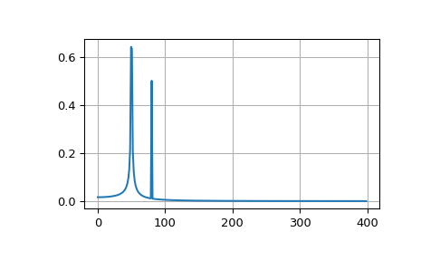
该示例绘制了两个正弦和的 FFT。

>>> from scipy.fft import fft, fftfreq
>>> import numpy as np
>>> # Number of sample points
>>> N = 600
>>> # sample spacing
>>> T = 1.0 / 800.0
>>> x = np.linspace(0.0, N*T, N, endpoint=False)
>>> y = np.sin(50.0 * 2.0*np.pi*x) + 0.5*np.sin(80.0 * 2.0*np.pi*x)
>>> yf = fft(y)
>>> xf = fftfreq(N, T)[:N//2]
>>> import matplotlib.pyplot as plt
>>> plt.plot(xf, 2.0/N * np.abs(yf[0:N//2]))
>>> plt.grid()
>>> plt.show()

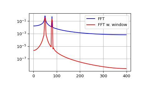
FFT 输入信号本质上是截断的。这种截断可以建模为无限信号与矩形窗函数的乘积。在频域中，这种乘积变成信号频谱与窗函数频谱的卷积，形式为 \(\sin(x)/x\)。这种卷积是称为频谱泄漏的效应的原因（请参见 [WPW]）。使用专用窗函数对信号进行加窗有助于减轻频谱泄漏。以下示例使用来自 scipy.signal 的 Blackman 窗，并显示了加窗的效果（出于说明目的，FFT 的零分量已被截断）。

>>> from scipy.fft import fft, fftfreq
>>> import numpy as np
>>> # Number of sample points
>>> N = 600
>>> # sample spacing
>>> T = 1.0 / 800.0
>>> x = np.linspace(0.0, N*T, N, endpoint=False)
>>> y = np.sin(50.0 * 2.0*np.pi*x) + 0.5*np.sin(80.0 * 2.0*np.pi*x)
>>> yf = fft(y)
>>> from scipy.signal.windows import blackman
>>> w = blackman(N)
>>> ywf = fft(y*w)
>>> xf = fftfreq(N, T)[:N//2]
>>> import matplotlib.pyplot as plt
>>> plt.semilogy(xf[1:N//2], 2.0/N * np.abs(yf[1:N//2]), '-b')
>>> plt.semilogy(xf[1:N//2], 2.0/N * np.abs(ywf[1:N//2]), '-r')
>>> plt.legend(['FFT', 'FFT w. window'])
>>> plt.grid()
>>> plt.show()

如果序列 x 是复值的，则频谱不再对称。为了简化 FFT 函数的使用，scipy 提供了以下两个帮助函数。

函数 fftfreq 返回 FFT 采样频率点。

>>> from scipy.fft import fftfreq
>>> freq = fftfreq(8, 0.125)
>>> freq
array([ 0., 1., 2., 3., -4., -3., -2., -1.])

类似地，函数 fftshift 允许交换向量的下半部分和上半部分，使其适合显示。

>>> from scipy.fft import fftshift
>>> x = np.arange(8)
>>> fftshift(x)
array([4, 5, 6, 7, 0, 1, 2, 3])

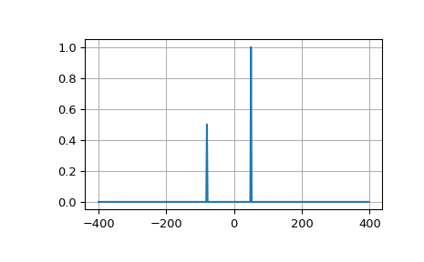
以下示例绘制了两个复指数的 FFT；请注意非对称频谱。

>>> from scipy.fft import fft, fftfreq, fftshift
>>> import numpy as np
>>> # number of signal points
>>> N = 400
>>> # sample spacing
>>> T = 1.0 / 800.0
>>> x = np.linspace(0.0, N*T, N, endpoint=False)
>>> y = np.exp(50.0 * 1.j * 2.0*np.pi*x) + 0.5*np.exp(-80.0 * 1.j * 2.0*np.pi*x)
>>> yf = fft(y)
>>> xf = fftfreq(N, T)
>>> xf = fftshift(xf)
>>> yplot = fftshift(yf)
>>> import matplotlib.pyplot as plt
>>> plt.plot(xf, 1.0/N * np.abs(yplot))
>>> plt.grid()
>>> plt.show()

函数 rfft 计算实序列的 FFT，并仅输出一半频率范围的复 FFT 系数 \(y[n]\)。对于实输入，其余的负频率分量由 FFT 的厄米特对称性暗示（y[n] = conj(y[-n])）。如果 N 是偶数：\([Re(y[0]) + 0j, y[1], ..., Re(y[N/2]) + 0j]\)；如果 N 是奇数 \([Re(y[0]) + 0j, y[1], ..., y[N/2]\)。明确显示为 \(Re(y[k]) + 0j\) 的项被限制为纯实数，因为根据厄米特性质，它们是它们自己的复共轭。

对应的函数 irfft 使用此特殊顺序计算 FFT 系数的 IFFT。

>>> from scipy.fft import fft, rfft, irfft
>>> x = np.array([1.0, 2.0, 1.0, -1.0, 1.5, 1.0])
>>> fft(x)
array([ 5.5 +0.j        ,  2.25-0.4330127j , -2.75-1.29903811j,
        1.5 +0.j        , -2.75+1.29903811j,  2.25+0.4330127j ])
>>> yr = rfft(x)
>>> yr
array([ 5.5 +0.j        ,  2.25-0.4330127j , -2.75-1.29903811j,
        1.5 +0.j        ])
>>> irfft(yr)
array([ 1. ,  2. ,  1. , -1. ,  1.5,  1. ])
>>> x = np.array([1.0, 2.0, 1.0, -1.0, 1.5])
>>> fft(x)
array([ 4.5       +0.j        ,  2.08155948-1.65109876j,
       -1.83155948+1.60822041j, -1.83155948-1.60822041j,
        2.08155948+1.65109876j])
>>> yr = rfft(x)
>>> yr
array([ 4.5       +0.j        ,  2.08155948-1.65109876j,
        -1.83155948+1.60822041j])

请注意，奇数和偶数长度信号的 rfft 具有相同的形状。默认情况下，irfft 假设输出信号的长度应该是偶数。因此，对于奇数信号，它将给出错误的结果

>>> irfft(yr)
array([ 1.70788987,  2.40843925, -0.37366961,  0.75734049])

要恢复原始的奇数长度信号，我们必须通过 n 参数传递输出形状。

>>> irfft(yr, n=len(x))
array([ 1. ,  2. ,  1. , -1. ,  1.5])

2 和 N 维离散傅立叶变换

函数 fft2 和 ifft2 分别提供 2 维 FFT 和 IFFT。类似地，fftn 和 ifftn 分别提供 N 维 FFT 和 IFFT。

对于实输入信号，类似于 rfft，我们有函数 rfft2 和 irfft2 用于 2 维实变换；rfftn 和 irfftn 用于 N 维实变换。

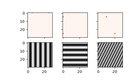
下面的示例演示了 2-D IFFT，并绘制了结果（2-D）时域信号。

>>> from scipy.fft import ifftn
>>> import matplotlib.pyplot as plt
>>> import matplotlib.cm as cm
>>> import numpy as np
>>> N = 30
>>> f, ((ax1, ax2, ax3), (ax4, ax5, ax6)) = plt.subplots(2, 3, sharex='col', sharey='row')
>>> xf = np.zeros((N,N))
>>> xf[0, 5] = 1
>>> xf[0, N-5] = 1
>>> Z = ifftn(xf)
>>> ax1.imshow(xf, cmap=cm.Reds)
>>> ax4.imshow(np.real(Z), cmap=cm.gray)
>>> xf = np.zeros((N, N))
>>> xf[5, 0] = 1
>>> xf[N-5, 0] = 1
>>> Z = ifftn(xf)
>>> ax2.imshow(xf, cmap=cm.Reds)
>>> ax5.imshow(np.real(Z), cmap=cm.gray)
>>> xf = np.zeros((N, N))
>>> xf[5, 10] = 1
>>> xf[N-5, N-10] = 1
>>> Z = ifftn(xf)
>>> ax3.imshow(xf, cmap=cm.Reds)
>>> ax6.imshow(np.real(Z), cmap=cm.gray)
>>> plt.show()

离散余弦变换

SciPy 提供了 DCT，函数为 dct，相应的 IDCT 函数为 idct。DCT 有 8 种类型 [WPC]、[Mak]；但是，scipy 中仅实现了前 4 种类型。“DCT”通常指 DCT 类型 2，“逆 DCT”通常指 DCT 类型 3。此外，DCT 系数可以以不同的方式进行归一化（对于大多数类型，scipy 提供 None 和 ortho）。dct/idct 函数调用的两个参数允许设置 DCT 类型和系数归一化。

对于单维数组 x，dct(x, norm=’ortho’) 等于 MATLAB dct(x)。

I 型 DCT

SciPy 使用以下未归一化 DCT-I 定义（norm=None）

\[y[k] = x_0 + (-1)^k x_{N-1} + 2\sum_{n=1}^{N-2} x[n] \cos\left(\frac{\pi nk}{N-1}\right), \qquad 0 \le k < N.\]

请注意，DCT-I 仅支持输入大小 > 1。

II 型 DCT

SciPy 使用以下未归一化 DCT-II 定义（norm=None）

\[y[k] = 2 \sum_{n=0}^{N-1} x[n] \cos \left({\pi(2n+1)k \over 2N} \right) \qquad 0 \le k < N.\]

对于归一化 DCT（norm='ortho'），DCT 系数 \(y[k]\) 乘以缩放因子 f

\[\begin{split}f = \begin{cases} \sqrt{1/(4N)}, & \text{如果 $k = 0$} \\ \sqrt{1/(2N)}, & \text{否则} \end{cases} \, .\end{split}\]

在这种情况下，DCT “基函数” \(\phi_k[n] = 2 f \cos \left({\pi(2n+1)k \over 2N} \right)\) 变成正交归一

\[\sum_{n=0}^{N-1} \phi_k[n] \phi_l[n] = \delta_{lk}.\]

III 型 DCT

SciPy 使用以下未归一化 DCT-III 定义（norm=None）

\[y[k] = x_0 + 2 \sum_{n=1}^{N-1} x[n] \cos\left({\pi n(2k+1) \over 2N}\right) \qquad 0 \le k < N,\]

或者，对于 norm='ortho'

\[y[k] = {x_0\over\sqrt{N}} + {2\over\sqrt{N}} \sum_{n=1}^{N-1} x[n] \cos\left({\pi n(2k+1) \over 2N}\right) \qquad 0 \le k < N.\]

IV 型 DCT

SciPy 使用以下未归一化 DCT-IV 定义（norm=None）

\[y[k] = 2 \sum_{n=0}^{N-1} x[n] \cos\left({\pi (2n+1)(2k+1) \over 4N}\right) \qquad 0 \le k < N,\]

或者，对于 norm='ortho'

\[y[k] = \sqrt{2\over N}\sum_{n=0}^{N-1} x[n] \cos\left({\pi (2n+1)(2k+1) \over 4N}\right) \qquad 0 \le k < N\]

DCT 和 IDCT

（未归一化）DCT-III 是（未归一化）DCT-II 的逆，乘以一个 2N 因子。正交归一化 DCT-III 正好是正交归一化 DCT-II 的逆。函数 idct 执行 DCT 和 IDCT 类型之间的映射，以及正确的归一化。

以下示例显示了不同类型和归一化下 DCT 和 IDCT 之间的关系。

>>> from scipy.fft import dct, idct
>>> x = np.array([1.0, 2.0, 1.0, -1.0, 1.5])

DCT-II 和 DCT-III 互为逆，因此对于正交归一化变换，我们返回到原始信号。

>>> dct(dct(x, type=2, norm='ortho'), type=3, norm='ortho')
array([ 1. ,  2. ,  1. , -1. ,  1.5])

然而，在默认归一化下执行相同的操作，我们会获得一个额外的缩放因子 \(2N=10\)，因为前向变换未归一化。

>>> dct(dct(x, type=2), type=3)
array([ 10.,  20.,  10., -10.,  15.])

出于此原因，我们应该对两者使用函数 idct，给出正确归一化的结果。

>>> # Normalized inverse: no scaling factor
>>> idct(dct(x, type=2), type=2)
array([ 1. ,  2. ,  1. , -1. ,  1.5])

对于 DCT-I，可以看出类似的结果，它是其自身的逆，乘以一个 \(2(N-1)\) 因子。

>>> dct(dct(x, type=1, norm='ortho'), type=1, norm='ortho')
array([ 1. ,  2. ,  1. , -1. ,  1.5])
>>> # Unnormalized round-trip via DCT-I: scaling factor 2*(N-1) = 8
>>> dct(dct(x, type=1), type=1)
array([ 8. ,  16.,  8. , -8. ,  12.])
>>> # Normalized inverse: no scaling factor
>>> idct(dct(x, type=1), type=1)
array([ 1. ,  2. ,  1. , -1. ,  1.5])

对于 DCT-IV，它也是其自身的逆，其因子为 \(2N\)。

>>> dct(dct(x, type=4, norm='ortho'), type=4, norm='ortho')
array([ 1. ,  2. ,  1. , -1. ,  1.5])
>>> # Unnormalized round-trip via DCT-IV: scaling factor 2*N = 10
>>> dct(dct(x, type=4), type=4)
array([ 10.,  20.,  10., -10.,  15.])
>>> # Normalized inverse: no scaling factor
>>> idct(dct(x, type=4), type=4)
array([ 1. ,  2. ,  1. , -1. ,  1.5])

示例

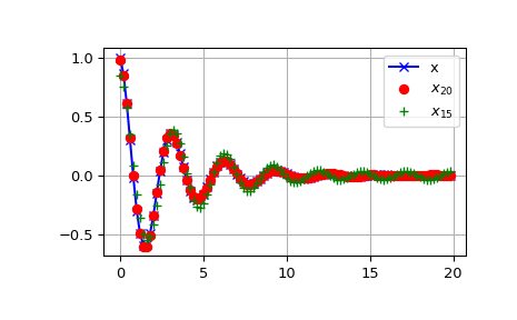
DCT 呈现出“能量压缩特性”，这意味着对于许多信号，只有前几个 DCT 系数具有显著幅度。将其他系数归零会导致较小的重构误差，这一事实被用于有损信号压缩（例如 JPEG 压缩）。

下面的示例显示了一个信号 x 和两个重构（\(x_{20}\) 和 \(x_{15}\)）来自信号的 DCT 系数。信号 \(x_{20}\) 由前 20 个 DCT 系数重构，\(x_{15}\) 由前 15 个 DCT 系数重构。可以看出，使用 20 个系数的相对误差仍然很小（~0.1%），但提供了五倍的压缩率。

>>> from scipy.fft import dct, idct
>>> import matplotlib.pyplot as plt
>>> N = 100
>>> t = np.linspace(0,20,N, endpoint=False)
>>> x = np.exp(-t/3)*np.cos(2*t)
>>> y = dct(x, norm='ortho')
>>> window = np.zeros(N)
>>> window[:20] = 1
>>> yr = idct(y*window, norm='ortho')
>>> sum(abs(x-yr)**2) / sum(abs(x)**2)
0.0009872817275276098
>>> plt.plot(t, x, '-bx')
>>> plt.plot(t, yr, 'ro')
>>> window = np.zeros(N)
>>> window[:15] = 1
>>> yr = idct(y*window, norm='ortho')
>>> sum(abs(x-yr)**2) / sum(abs(x)**2)
0.06196643004256714
>>> plt.plot(t, yr, 'g+')
>>> plt.legend(['x', '$x_{20}$', '$x_{15}$'])
>>> plt.grid()
>>> plt.show()

离散正弦变换

SciPy 提供了 DST [Mak]，其函数为 dst，以及一个对应的 IDST，其函数为 idst。

理论上，DST 有 8 种类型，用于偶/奇边界条件和边界偏移的不同组合 [WPS]，只有前 4 种类型在 scipy 中实现。

I 型 DST

DST-I 假设输入在 n=-1 和 n=N 处为奇数。SciPy 使用以下未归一化的 DST-I 定义（norm=None）

\[y[k] = 2\sum_{n=0}^{N-1} x[n] \sin\left( \pi {(n+1) (k+1)}\over{N+1} \right), \qquad 0 \le k < N.\]

另请注意，DST-I 仅支持输入大小 > 1。未归一化的 DST-I 是其自身的逆，其系数为 2(N+1)。

II 型 DST

DST-II 假设输入在 n=-1/2 附近为奇数，在 n=N 附近为偶数。SciPy 使用以下未归一化 DST-II 定义 (norm=None)

\[y[k] = 2 \sum_{n=0}^{N-1} x[n] \sin\left( {\pi (n+1/2)(k+1)} \over N \right), \qquad 0 \le k < N.\]

III 型 DST

DST-III 假设输入在 n=-1 附近为奇数，在 n=N-1 附近为偶数。SciPy 使用以下未归一化 DST-III 定义 (norm=None)

\[y[k] = (-1)^k x[N-1] + 2 \sum_{n=0}^{N-2} x[n] \sin \left( {\pi (n+1)(k+1/2)} \over N \right), \qquad 0 \le k < N.\]

IV 型 DST

SciPy 使用以下未归一化 DST-IV 定义 (norm=None)

\[y[k] = 2 \sum_{n=0}^{N-1} x[n] \sin\left({\pi (2n+1)(2k+1) \over 4N}\right) \qquad 0 \le k < N,\]

或者，对于 norm='ortho'

\[y[k] = \sqrt{2\over N}\sum_{n=0}^{N-1} x[n] \sin\left({\pi (2n+1)(2k+1) \over 4N}\right) \qquad 0 \le k < N,\]

DST 和 IDST

以下示例显示了不同类型和归一化情况下 DST 和 IDST 之间的关系。

>>> from scipy.fft import dst, idst
>>> x = np.array([1.0, 2.0, 1.0, -1.0, 1.5])

DST-II 和 DST-III 互为逆，因此对于正交变换，我们返回原始信号。

>>> dst(dst(x, type=2, norm='ortho'), type=3, norm='ortho')
array([ 1. ,  2. ,  1. , -1. ,  1.5])

然而，在默认归一化下执行相同的操作，我们会获得一个额外的缩放因子 \(2N=10\)，因为前向变换未归一化。

>>> dst(dst(x, type=2), type=3)
array([ 10.,  20.,  10., -10.,  15.])

因此，我们应使用函数 idst，对两者使用相同的类型，从而提供正确归一化的结果。

>>> idst(dst(x, type=2), type=2)
array([ 1. ,  2. ,  1. , -1. ,  1.5])

对于 DST-I，可以观察到类似的结果，它本身就是其自身的逆，乘以一个因子 \(2(N-1)\)。

>>> dst(dst(x, type=1, norm='ortho'), type=1, norm='ortho')
array([ 1. ,  2. ,  1. , -1. ,  1.5])
>>>  # scaling factor 2*(N+1) = 12
>>> dst(dst(x, type=1), type=1)
array([ 12.,  24.,  12., -12.,  18.])
>>>  # no scaling factor
>>> idst(dst(x, type=1), type=1)
array([ 1. ,  2. ,  1. , -1. ,  1.5])

对于 DST-IV，它也是其自身的逆，乘以一个因子 \(2N\)。

>>> dst(dst(x, type=4, norm='ortho'), type=4, norm='ortho')
array([ 1. ,  2. ,  1. , -1. ,  1.5])
>>>  # scaling factor 2*N = 10
>>> dst(dst(x, type=4), type=4)
array([ 10.,  20.,  10., -10.,  15.])
>>>  # no scaling factor
>>> idst(dst(x, type=4), type=4)
array([ 1. ,  2. ,  1. , -1. ,  1.5])

快速汉克尔变换

SciPy 提供了函数 fht 和 ifht 来对对数间隔输入数组执行快速汉克尔变换 (FHT) 及其逆变换 (IFHT)。

FHT 是连续汉克尔变换的离散化版本，由 [Ham00] 定义：

\[A(k) = \int_{0}^{\infty} \! a(r) \, J_{\mu}(kr) \, k \, dr \;,\]

其中 \(J_{\mu}\) 是阶数为 \(\mu\) 的贝塞尔函数。在变量 \(r \to \log r\)、\(k \to \log k\) 变化下，这变为

\[A(e^{\log k}) = \int_{0}^{\infty} \! a(e^{\log r}) \, J_{\mu}(e^{\log k + \log r}) \, e^{\log k + \log r} \, d{\log r}\]

这是对数空间中的卷积。FHT 算法使用 FFT 在离散输入数据上执行此卷积。

必须小心，以最大程度地减少由于 FFT 卷积的循环性质而产生的数值振铃。为了确保低振铃条件 [Ham00] 成立，可以使用 fhtoffset 函数计算的偏移量稍微偏移输出数组。

参考

[CT65]

Cooley, James W. 和 John W. Tukey，1965 年，“一种用于机器计算复杂傅里叶级数的算法”，Math. Comput. 19: 297-301。

[NR07]

Press, W.、Teukolsky, S.、Vetterline, W.T. 和 Flannery, B.P.，2007 年，数值食谱：科学计算的艺术，第 12-13 章。剑桥大学出版社，英国剑桥。

[Mak] (1,2)

J. Makhoul，1980 年，“一维和二维快速余弦变换”，IEEE 声学、语音和信号处理事务第 28 卷（1），第 27-34 页，DOI:10.1109/TASSP.1980.1163351

[Ham00] (1,2)

A. J. S. Hamilton，2000 年，“非线性功率谱的非相关模式”，MNRAS，312，257。 DOI:10.1046/j.1365-8711.2000.03071.x

[WPW]

https://en.wikipedia.org/wiki/Window_function

[WPC]

https://en.wikipedia.org/wiki/Discrete_cosine_transform

[WPS]

https://en.wikipedia.org/wiki/Discrete_sine_transform