一维插值#
分段线性插值#
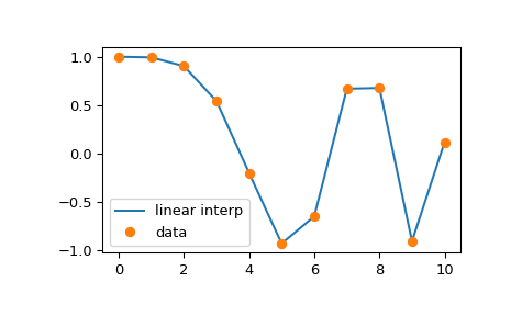
如果你只需要线性(也称为折线)插值,可以使用 numpy.interp 函数。它接受两个用于插值的数组数据,x 和 y,以及第三个数组,xnew,用于评估插值
>>> import numpy as np
>>> x = np.linspace(0, 10, num=11)
>>> y = np.cos(-x**2 / 9.0)
构建插值
>>> xnew = np.linspace(0, 10, num=1001)
>>> ynew = np.interp(xnew, x, y)
并绘制它
>>> import matplotlib.pyplot as plt
>>> plt.plot(xnew, ynew, '-', label='linear interp')
>>> plt.plot(x, y, 'o', label='data')
>>> plt.legend(loc='best')
>>> plt.show()
三次样条#
当然,分段线性插值在数据点处产生角点,线性段在此处连接。为了产生更平滑的曲线,可以使用三次样条,其中插值曲线由具有匹配一阶和二阶导数的三次段组成。在代码中,这些对象通过 CubicSpline 类实例表示。实例使用 x 和 y 数组数据构建,然后可以使用目标 xnew 值进行评估
>>> from scipy.interpolate import CubicSpline
>>> spl = CubicSpline([1, 2, 3, 4, 5, 6], [1, 4, 8, 16, 25, 36])
>>> spl(2.5)
5.57
CubicSpline 对象的 __call__ 方法接受标量值和数组。它还接受第二个参数,nu,用于评估 nu 阶导数。例如,我们绘制样条的导数
>>> from scipy.interpolate import CubicSpline
>>> x = np.linspace(0, 10, num=11)
>>> y = np.cos(-x**2 / 9.)
>>> spl = CubicSpline(x, y)
>>> import matplotlib.pyplot as plt
>>> fig, ax = plt.subplots(4, 1, figsize=(5, 7))
>>> xnew = np.linspace(0, 10, num=1001)
>>> ax[0].plot(xnew, spl(xnew))
>>> ax[0].plot(x, y, 'o', label='data')
>>> ax[1].plot(xnew, spl(xnew, nu=1), '--', label='1st derivative')
>>> ax[2].plot(xnew, spl(xnew, nu=2), '--', label='2nd derivative')
>>> ax[3].plot(xnew, spl(xnew, nu=3), '--', label='3rd derivative')
>>> for j in range(4):
...     ax[j].legend(loc='best')
>>> plt.tight_layout()
>>> plt.show()
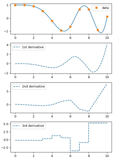
请注意,一阶和二阶导数在构造时是连续的,而三阶导数在数据点处跳跃。
单调插值器#
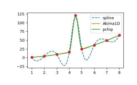
三次样条曲线在构造上是两次连续可微的。这可能导致样条函数在数据点之间振荡和“过冲”。在这些情况下,可以使用所谓的*单调*三次插值器作为替代:这些插值器被构造为仅一次连续可微,并试图保留数据所隐含的局部形状。 scipy.interpolate 提供了两种此类对象: PchipInterpolator 和 Akima1DInterpolator 。为了说明,让我们考虑一个包含异常值的数据
>>> from scipy.interpolate import CubicSpline, PchipInterpolator, Akima1DInterpolator
>>> x = np.array([1., 2., 3., 4., 4.5, 5., 6., 7., 8])
>>> y = x**2
>>> y[4] += 101
>>> import matplotlib.pyplot as plt
>>> xx = np.linspace(1, 8, 51)
>>> plt.plot(xx, CubicSpline(x, y)(xx), '--', label='spline')
>>> plt.plot(xx, Akima1DInterpolator(x, y)(xx), '-', label='Akima1D')
>>> plt.plot(xx, PchipInterpolator(x, y)(xx), '-', label='pchip')
>>> plt.plot(x, y, 'o')
>>> plt.legend()
>>> plt.show()
使用 B 样条曲线进行插值#
B 样条曲线是分段多项式的另一种(如果形式上等效)表示。这种基通常比幂基在计算上更稳定,并且适用于各种应用,包括插值、回归和曲线表示。详细信息在 分段多项式部分 中给出,这里我们通过构造正弦函数的插值来说明它们的用法
>>> x = np.linspace(0, 3/2, 7)
>>> y = np.sin(np.pi*x)
为了构造给定数据数组的插值对象,x 和 y,我们使用 make_interp_spline 函数
>>> from scipy.interpolate import make_interp_spline
>>> bspl = make_interp_spline(x, y, k=3)
此函数返回一个对象,该对象具有与 CubicSpline 对象类似的接口。特别是,它可以在数据点处进行评估和微分
>>> der = bspl.derivative()      # a BSpline representing the derivative
>>> import matplotlib.pyplot as plt
>>> xx = np.linspace(0, 3/2, 51)
>>> plt.plot(xx, bspl(xx), '--', label=r'$\sin(\pi x)$ approx')
>>> plt.plot(x, y, 'o', label='data')
>>> plt.plot(xx, der(xx)/np.pi, '--', label='$d \sin(\pi x)/dx / \pi$ approx')
>>> plt.legend()
>>> plt.show()
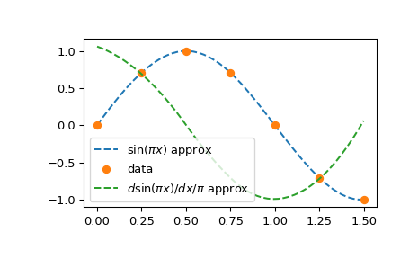
请注意,通过在 make_interp_spline 调用中指定 k=3,我们请求了一个三次样条曲线(这是默认值,因此可以省略 k=3);三次函数的导数是二次函数
>>> bspl.k, der.k
(3, 2)
默认情况下,make_interp_spline(x, y) 的结果等效于 CubicSpline(x, y)。区别在于前者允许一些可选功能:它可以通过可选参数 k 构造不同阶数的样条曲线,并通过可选参数 t 预定义节点。
样条插值的边界条件可以通过 bc_type 参数控制,该参数用于 make_interp_spline 函数和 CubicSpline 构造函数。默认情况下,两者都使用“非节点”边界条件。
参数样条曲线#
到目前为止,我们考虑的是样条函数,其中数据 y 预计显式地依赖于自变量 x——因此插值函数满足 \(f(x_j) = y_j\)。样条曲线将 x 和 y 数组视为平面上点的坐标,\(\mathbf{p}_j\),并且通过这些点的插值曲线由一些额外的参数(通常称为 u)参数化。请注意,这种构造很容易推广到更高维度,其中 \(\mathbf{p}_j\) 是 N 维空间中的点。
样条曲线可以使用插值函数处理多维数据数组这一事实轻松构建。与数据点相对应的参数 u 的值需要由用户单独提供。
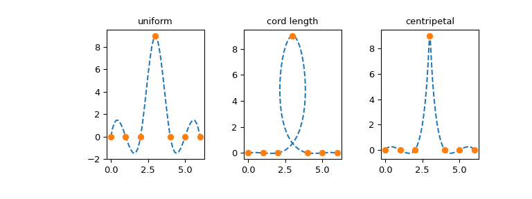
参数化的选择取决于问题,不同的参数化可能会产生截然不同的曲线。例如,我们考虑了(一个有点困难的)数据集的三个参数化,这些数据集取自 Ref [1] 第 6 章,该参考文献列在 BSpline 文档字符串中
>>> x = [0, 1, 2, 3, 4, 5, 6]
>>> y = [0, 0, 0, 9, 0, 0, 0]
>>> p = np.stack((x, y))
>>> p
array([[0, 1, 2, 3, 4, 5, 6],
       [0, 0, 0, 9, 0, 0, 0]])
我们将 p 数组中的元素作为平面上的七个点的坐标,其中 p[:, j] 给出了点 \(\mathbf{p}_j\) 的坐标。
首先,考虑均匀参数化,\(u_j = j\)
>>> u_unif = x
其次,我们考虑所谓的弦长参数化,它不过是连接数据点的直线段的累积长度
对于 \(j=1, 2, \dots\) 和 \(u_0 = 0\)。这里 \(| \cdots |\) 是平面上的连续点 \(p_j\) 之间的距离。
>>> dp = p[:, 1:] - p[:, :-1]      # 2-vector distances between points
>>> l = (dp**2).sum(axis=0)        # squares of lengths of 2-vectors between points
>>> u_cord = np.sqrt(l).cumsum()   # cumulative sums of 2-norms
>>> u_cord = np.r_[0, u_cord]      # the first point is parameterized at zero
最后,我们考虑有时被称为向心参数化:\(u_j = u_{j-1} + |\mathbf{p}_j - \mathbf{p}_{j-1}|^{1/2}\)。由于多了平方根,连续值 \(u_j - u_{j-1}\) 之间的差值将小于弦长参数化。
>>> u_c = np.r_[0, np.cumsum((dp**2).sum(axis=0)**0.25)]
现在绘制结果曲线
>>> from scipy.interpolate import make_interp_spline
>>> import matplotlib.pyplot as plt
>>> fig, ax = plt.subplots(1, 3, figsize=(8, 3))
>>> parametrizations = ['uniform', 'cord length', 'centripetal']
>>>
>>> for j, u in enumerate([u_unif, u_cord, u_c]):
...    spl = make_interp_spline(u, p, axis=1)    # note p is a 2D array
...
...    uu = np.linspace(u[0], u[-1], 51)
...    xx, yy = spl(uu)
...
...    ax[j].plot(xx, yy, '--')
...    ax[j].plot(p[0, :], p[1, :], 'o')
...    ax[j].set_title(parametrizations[j])
>>> plt.show()
1-D 插值的传统接口 (interp1d)#
注意
interp1d 被认为是传统 API,不建议在新的代码中使用。请考虑使用更具体的插值器。
interp1d 类在 scipy.interpolate 中是一个方便的方法,用于基于固定数据点创建函数,该函数可以使用线性插值在给定数据定义的域内的任何地方进行评估。此类的实例是通过传递包含数据的 1-D 向量来创建的。此类的实例定义了一个 __call__ 方法,因此可以像一个函数一样对待它,该函数在已知数据值之间进行插值以获得未知值。边界处的行为可以在实例化时指定。以下示例演示了它的使用,用于线性插值和三次样条插值
>>> from scipy.interpolate import interp1d
>>> x = np.linspace(0, 10, num=11, endpoint=True)
>>> y = np.cos(-x**2/9.0)
>>> f = interp1d(x, y)
>>> f2 = interp1d(x, y, kind='cubic')
>>> xnew = np.linspace(0, 10, num=41, endpoint=True)
>>> import matplotlib.pyplot as plt
>>> plt.plot(x, y, 'o', xnew, f(xnew), '-', xnew, f2(xnew), '--')
>>> plt.legend(['data', 'linear', 'cubic'], loc='best')
>>> plt.show()
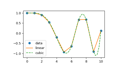
“cubic”类型的interp1d 等效于make_interp_spline,而“linear”类型等效于numpy.interp,同时还允许 N 维的 y 数组。
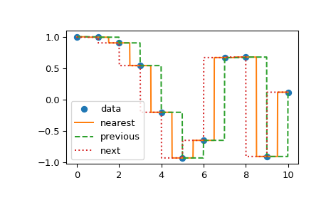
在interp1d 中,另一组插值是 nearest、previous 和 next,它们分别返回 x 轴上最接近的、之前的或下一个点。Nearest 和 next 可以被认为是因果插值滤波器的一种特殊情况。以下示例演示了它们的用法,使用与上一个示例相同的数据。
>>> from scipy.interpolate import interp1d
>>> x = np.linspace(0, 10, num=11, endpoint=True)
>>> y = np.cos(-x**2/9.0)
>>> f1 = interp1d(x, y, kind='nearest')
>>> f2 = interp1d(x, y, kind='previous')
>>> f3 = interp1d(x, y, kind='next')
>>> xnew = np.linspace(0, 10, num=1001, endpoint=True)
>>> import matplotlib.pyplot as plt
>>> plt.plot(x, y, 'o')
>>> plt.plot(xnew, f1(xnew), '-', xnew, f2(xnew), '--', xnew, f3(xnew), ':')
>>> plt.legend(['data', 'nearest', 'previous', 'next'], loc='best')
>>> plt.show()
缺失数据#
我们注意到scipy.interpolate 不支持带有缺失数据的插值。表示缺失数据的两种常用方法是使用numpy.ma 库的掩码数组,以及将缺失值编码为非数字,NaN。
这两种方法都没有得到 scipy.interpolate 的直接支持。个别例程可能提供部分支持或变通方法,但总的来说,该库严格遵守 IEEE 754 语义,其中 NaN 表示非数字,即非法数学运算的结果(例如除以零),而不是缺失。