scipy.stats.
bayes_mvs#
- scipy.stats.bayes_mvs(data, alpha=0.9)[source]#
均值、方差和标准差的贝叶斯置信区间。
- 参数:
- **data**array_like
输入数据,如果多维,则由
bayes_mvs平铺为一维。要求至少 2 个数据点。- **alpha**float, 可选
返回的置信区间包含真实参数的概率。
- 返回:
- **mean_cntr, var_cntr, std_cntr**元组
三个结果分别用于均值、方差和标准差。每个结果都是一个元组,形式为
(center, (lower, upper))
其中 center 是给定数据的条件 pdf 的值的均值,而 (lower, upper) 是一个置信区间,以中位数为中心,包含估计值为概率
alpha。
另请参阅
注释
每个均值、方差和标准差估计值的元组都代表 (center, (lower, upper)),其中 center 是给定数据的条件 pdf 的值的均值,而 (lower, upper) 是一个置信区间,以中位数为中心,包含估计值为概率
alpha。将数据转换为一维,并假设所有数据具有相同的均值和方差。对于方差和标准差使用杰弗里斯先验。
等效于
tuple((x.mean(), x.interval(alpha)) for x in mvsdist(dat))参考文献
T.E. Oliphant,“从数据估计均值、方差和标准差的贝叶斯视角”,https://scholarsarchive.byu.edu/facpub/278,2006 年。
示例
首先是一个基本示例,用于演示输出
>>> from scipy import stats
>>> data = [6, 9, 12, 7, 8, 8, 13]
>>> mean, var, std = stats.bayes_mvs(data)
>>> mean
Mean(statistic=9.0, minmax=(7.103650222612533, 10.896349777387467))
>>> var
Variance(statistic=10.0, minmax=(3.176724206, 24.45910382))
>>> std
Std_dev(statistic=2.9724954732045084,
        minmax=(1.7823367265645143, 4.945614605014631))
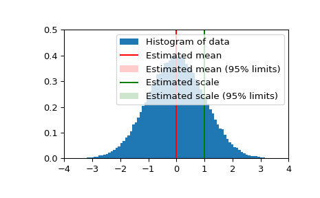
现在,我们生成一些正态分布的随机数据,并获得均值和标准差的估计值,以及这些估计值的 95% 置信区间
>>> n_samples = 100000
>>> data = stats.norm.rvs(size=n_samples)
>>> res_mean, res_var, res_std = stats.bayes_mvs(data, alpha=0.95)
>>> import matplotlib.pyplot as plt
>>> fig = plt.figure()
>>> ax = fig.add_subplot(111)
>>> ax.hist(data, bins=100, density=True, label='Histogram of data')
>>> ax.vlines(res_mean.statistic, 0, 0.5, colors='r', label='Estimated mean')
>>> ax.axvspan(res_mean.minmax[0],res_mean.minmax[1], facecolor='r',
...            alpha=0.2, label=r'Estimated mean (95% limits)')
>>> ax.vlines(res_std.statistic, 0, 0.5, colors='g', label='Estimated scale')
>>> ax.axvspan(res_std.minmax[0],res_std.minmax[1], facecolor='g', alpha=0.2,
...            label=r'Estimated scale (95% limits)')
>>> ax.legend(fontsize=10)
>>> ax.set_xlim([-4, 4])
>>> ax.set_ylim([0, 0.5])
>>> plt.show()